Chapter 4 Taller RASTER Y CUBOS DE DATOS VECTORIALES: Aplicación de software de información geográfica y modelado
gracias Amanda Rehbein <3 (amanda.rehbein@usp.br)
Raster son informacion espaciales en una grilla espacial. En general, la informacion de las frillas tiene una distancia homogenea, Por ejemplo, vea las siguientes figuras:
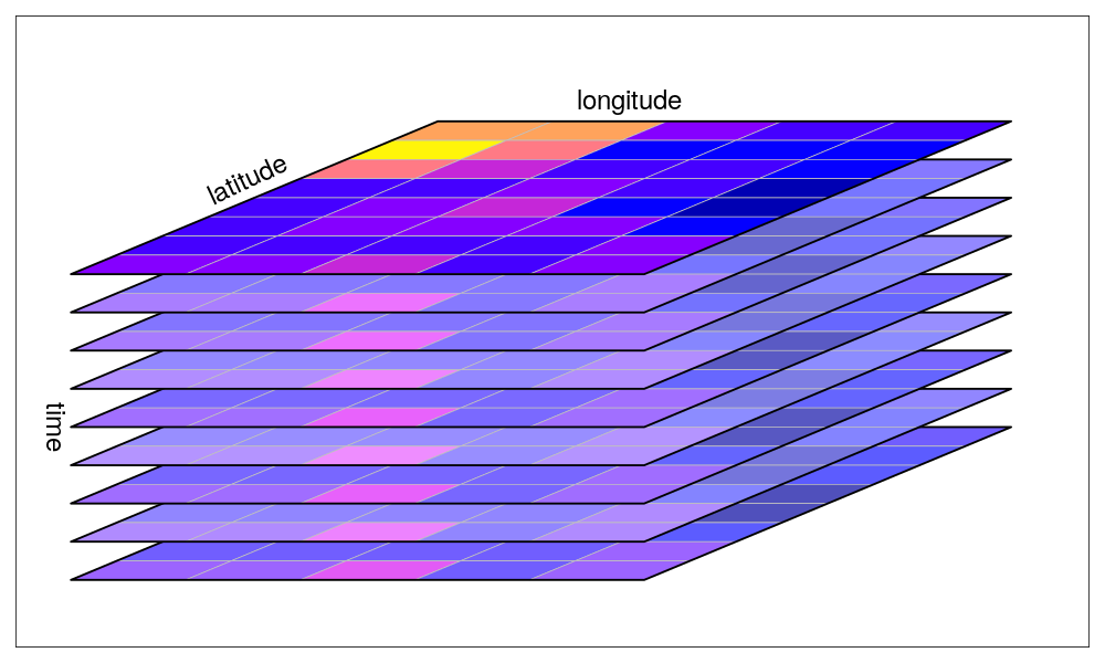
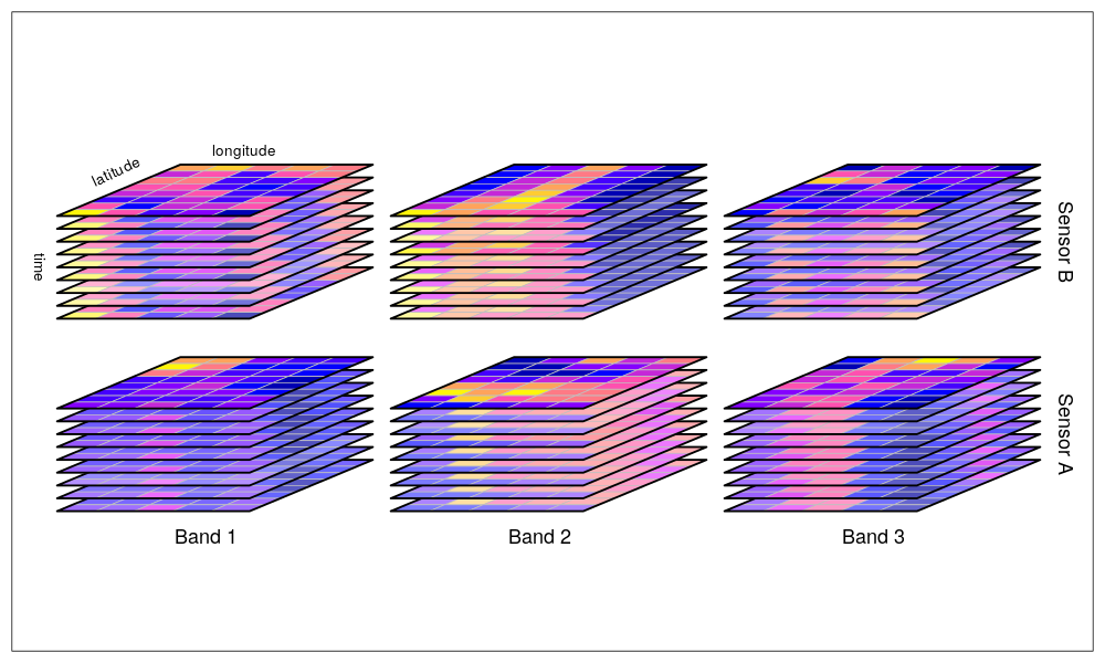
Por ejemplo, cada banda podria representar un tiempo. Como se ve, estos ne realidad son cubos de datos de varias dimensiones, sin embargo, pueden existir grillas irregulares, como las que osn bien represnetadas con el paquete stars
Preparense, porque vamos a avanzar directamente en el fondo del mundo de los datos espacio/temporales grillados raster y stars
raster es una clase y una libreria de R que representa datos en grillas, llamados raster
stasr es una clase y una libreria de R que representa datos en grillas, llamados tambien rasters.
Por lo tanto, stars y raster tienen conexiones para leer los datos en formato GDAL raster. Que quiere decir esto????
Quiere decir que, tal como GDAL lee vectores, tambien lee [raster]((https://gdal.org/drivers/raster/index.html).: Coomopor ejemplo:
Vamos meterle manos a la obra, vamos a nadar en el mundo multidimensional de los raster y si no saben nadar aprenderan como los pajaros que aprenden ante la subita e inherente necesidada vital de sobrevivir.
Antes de abrir los datos con los programas, vamos a ver que vamos tenemos
## File dados/pr_Amon_HadGEM2-ES_historical_r1i1p1_DJF_1985-2004.nc (NC_FORMAT_CLASSIC):
##
##      4 variables (excluding dimension variables):
##         double lon_bnds[bnds,lon]
##         double lat_bnds[bnds,lat]
##         double time_bnds[bnds,time]
##         double pr[lon,lat,time]
##             standard_name: precipitation_flux
##             long_name: Precipitation
##             units: kg m-2 s-1
##             _FillValue: 1.00000002004088e+20
##             missing_value: 1.00000002004088e+20
##             comment: at surface; includes both liquid and solid phases from all types of clouds (both large-scale and convective)
##             original_name: mo: m01s05i216
##             history: 2011-03-22T15:05:23 out-of-bounds adjustments: (-1e-07 <= x < 0.0) => set to 0.0 2011-03-22T15:05:23Z altered by CMOR: replaced missing value flag (-1.07374e+09) with standard missing value (1e+20).
##             cell_methods: time: mean
##             associated_files: baseURL: http://cmip-pcmdi.llnl.gov/CMIP5/dataLocation gridspecFile: gridspec_atmos_fx_HadGEM2-ES_historical_r0i0p0.nc areacella: areacella_fx_HadGEM2-ES_historical_r0i0p0.nc
##
##      4 dimensions:
##         lon  Size:192
##             standard_name: longitude
##             long_name: longitude
##             units: degrees_east
##             axis: X
##             bounds: lon_bnds
##         bnds  Size:2
##         lat  Size:145
##             standard_name: latitude
##             long_name: latitude
##             units: degrees_north
##             axis: Y
##             bounds: lat_bnds
##         time  Size:19   *** is unlimited ***
##             standard_name: time
##             long_name: time
##             bounds: time_bnds
##             units: days since 1859-12-1 00:00:00
##             calendar: 360_day
##             axis: T
##
##     30 global attributes:
##         CDI: Climate Data Interface version ?? (http://mpimet.mpg.de/cdi)
##         Conventions: CF-1.4
##         history: Sun Sep 08 00:37:13 2019: cdo selmon,1 tmp_SELTIME_SEASSUM_pr_Amon_HadGEM2-ES_historical_r1i1p1_198412-200511.nc pr_Amon_HadGEM2-ES_historical_r1i1p1_DJF_1986-2004.nc
## Sun Sep 08 00:36:18 2019: cdo selyear,1986,1987,1988,1989,1990,1991,1992,1993,1994,1995,1996,1997,1998,1999,2000,2001,2002,2003,2004 tmp_SEASSUM_pr_Amon_HadGEM2-ES_historical_r1i1p1_198412-200511.nc tmp_SELTIME_SEASSUM_pr_Amon_HadGEM2-ES_historical_r1i1p1_198412-200511.nc
## Sun Sep 08 00:33:38 2019: cdo -b 64 seassum pr_Amon_HadGEM2-ES_historical_r1i1p1_198412-200511.nc tmp_SEASSUM_pr_Amon_HadGEM2-ES_historical_r1i1p1_198412-200511.nc
## MOHC pp to CMOR/NetCDF convertor (version 1.7.0) 2011-03-22T15:05:17Z CMOR rewrote data to comply with CF standards and CMIP5 requirements.
##         source: HadGEM2-ES (2009) atmosphere: HadGAM2 (N96L38); ocean: HadGOM2 (lat: 1.0-0.3 lon: 1.0 L40); land-surface/vegetation: MOSES2 and TRIFFID; tropospheric chemistry: UKCA; ocean biogeochemistry: diat-HadOCC
##         institution: Met Office Hadley Centre, Fitzroy Road, Exeter, Devon, EX1 3PB, UK, (http://www.metoffice.gov.uk)
##         institute_id: MOHC
##         experiment_id: historical
##         model_id: HadGEM2-ES
##         forcing: GHG, SA, Oz, LU, Sl, Vl, BC, OC, (GHG = CO2, N2O, CH4, CFCs)
##         parent_experiment_id: piControl
##         parent_experiment_rip: r1i1p1
##         branch_time: 0
##         contact: chris.d.jones@metoffice.gov.uk, michael.sanderson@metoffice.gov.uk
##         references: Bellouin N. et al, (2007) Improved representation of aerosols for HadGEM2. Meteorological Office Hadley Centre, Technical Note 73, March 2007; Collins W.J.  et al, (2008) Evaluation of the HadGEM2 model. Meteorological Office Hadley Centre, Technical Note 74,; Johns T.C. et al, (2006) The new Hadley Centre climate model HadGEM1: Evaluation of coupled simulations. Journal of Climate, American Meteorological Society, Vol. 19, No. 7, pages 1327-1353.; Martin G.M. et al, (2006) The physical properties of the atmosphere in the new Hadley Centre Global Environmental Model, HadGEM1 - Part 1: Model description and global climatology. Journal of Climate, American Meteorological Society, Vol. 19, No.7, pages 1274-1301.; Ringer M.A. et al, (2006) The physical properties of the atmosphere in the new Hadley Centre Global Environmental Model, HadGEM1 - Part 2: Aspects of variability and regional climate. Journal of Climate, American Meteorological Society, Vol. 19, No. 7, pages 1302-1326.
##         initialization_method: 1
##         physics_version: 1
##         tracking_id: 15cb947c-34d2-4da2-b830-9dd0123d96d3
##         mo_runid: ajhoh
##         product: output
##         experiment: historical
##         frequency: mon
##         creation_date: 2011-03-22T19:30:17Z
##         project_id: CMIP5
##         table_id: Table Amon (06 January 2011) 085e3f5c098d203b2fd5d296226f41b3
##         title: HadGEM2-ES model output prepared for CMIP5 historical
##         parent_experiment: pre-industrial control
##         modeling_realm: atmos
##         realization: 1
##         cmor_version: 2.5.3
## CDO: Climate Data Operators version 1.7.2 (http://mpimet.mpg.de/cdo)library(stars)
pcp_era5 <- read_stars("dados/pr_Amon_HadGEM2-ES_historical_r1i1p1_DJF_1985-2004.nc")
names(pcp_era5)
str(pcp_era5)
head(pcp_era5)brick es como literalmente un ladrillo considerndo usualmente la dimension tempral como un ladrillo.
como vemos, la funcion str entrega mucha informacion. Esta funcion no es comunmente usada, pero su archivo de documentacion es ?str
ERA5, investiguen!
Vamos a plotear estos datos!
## Loading required package: abindlibrary(cptcity)
pcp_era5 <- read_stars("dados/pr_Amon_HadGEM2-ES_historical_r1i1p1_DJF_1985-2004.nc")
plot(pcp_era5,
col = lucky(),
axes = TRUE)## Colour gradient: jjg_cbac_div_cbacRdYlGn03, number: 3683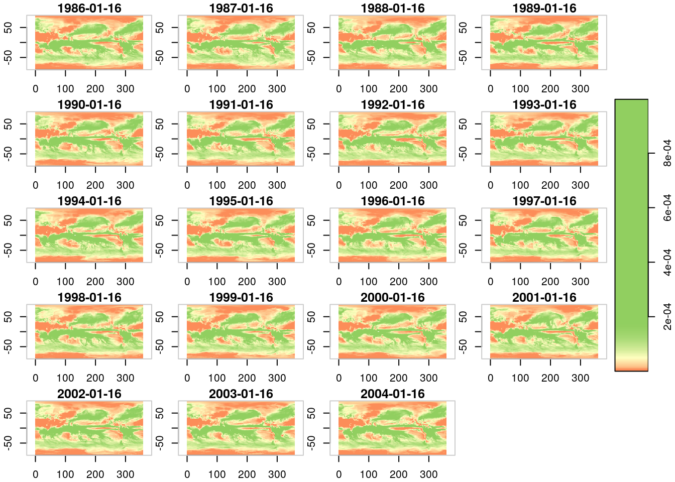
Ahora vamos voy a mostrar todo un script para hacer graficos y analizar datos climaticos usando la libreria raster
# ------------------------------------#
# Precipitacion y temperatura medias  #
#         Verano y invierno           #
#       (very simple analysis)        #
# ------------------------------------#

library(raster)
## Loading required package: splibrary(cptcity)
path <- "dados"
# DJF - VERANO: ####
# Open the precipitation file:
pcp_era5 <- brick("dados/r_ERA5_pcp_DJF_1985-2004.nc")
# Print information and metadata:
pcp_era5 # This file has 17 layers (years)## class : RasterBrick
## dimensions : 145, 192, 27840, 21 (nrow, ncol, ncell, nlayers)
## resolution : 1.875, 1.25 (x, y)
## extent : -0.9375, 359.0625, -90.625, 90.625 (xmin, xmax, ymin, ymax)
## crs : +proj=longlat +datum=WGS84 +ellps=WGS84 +towgs84=0,0,0
## source : /home/sergio/Documents/UBA/dados/r_ERA5_pcp_DJF_1985-2004.nc
## names : X1984.01.16.12.06.28, X1985.01.01.00.06.28, X1986.01.01.01.06.28, X1987.01.01.01.06.28, X1988.01.01.01.06.28, X1989.01.01.01.06.28, X1990.01.01.01.06.28, X1991.01.01.01.06.28, X1992.01.01.01.06.28, X1993.01.01.01.06.28, X1994.01.01.01.06.28, X1995.01.01.01.06.28, X1996.01.01.01.06.28, X1997.01.01.01.06.28, X1998.01.01.01.06.28, ...
## Date/time : 1984-01-16 12:06:28, 2005-12-01 01:06:28 (min, max)
## varname : mtpr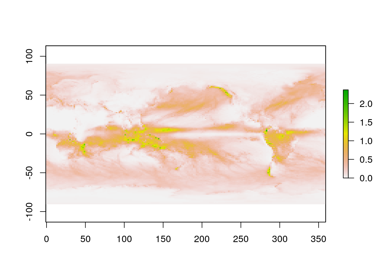
# Calculate the mean:
mean_pcp_era <- mean(pcp_era5*3600)

# Opening CMIP5 data model: HadGEM2-ES\
pcp_historical <- brick("dados/pr_Amon_HadGEM2-ES_historical_r1i1p1_DJF_1985-2004.nc")
plot(pcp_historical[[1]]*3600)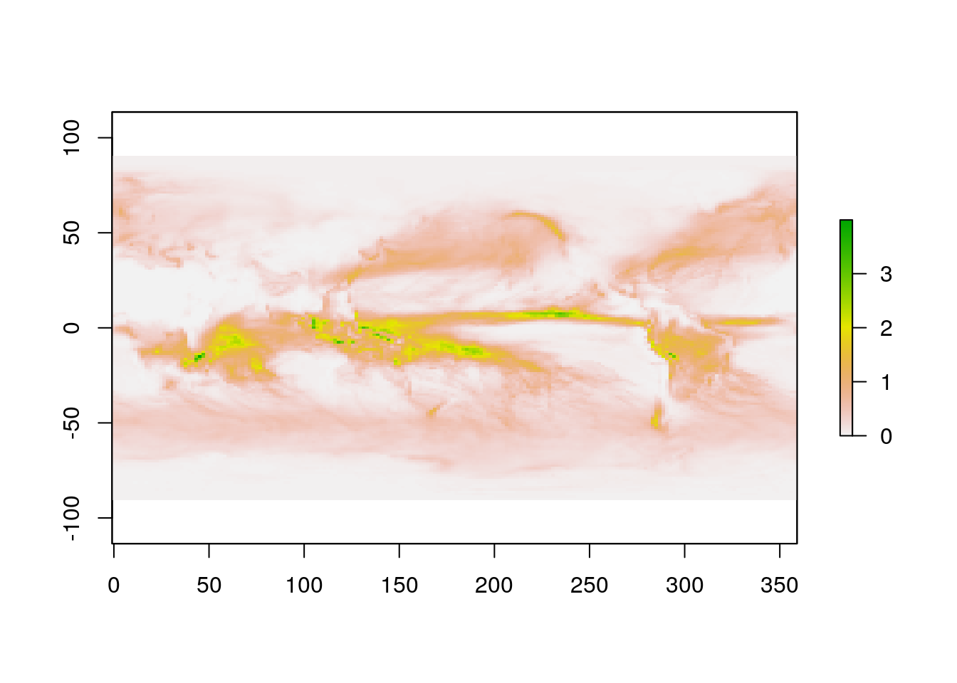
# calculando a media
mean_pcp_historical <- mean(pcp_historical)

spplot(mean_pcp_era, interpolate = T,
            main = "Observed Precipitation [mm/h] (ERA5) \n DJF (1985 - 2004)",
            col.regions = cpt("ncl_precip2_17lev"))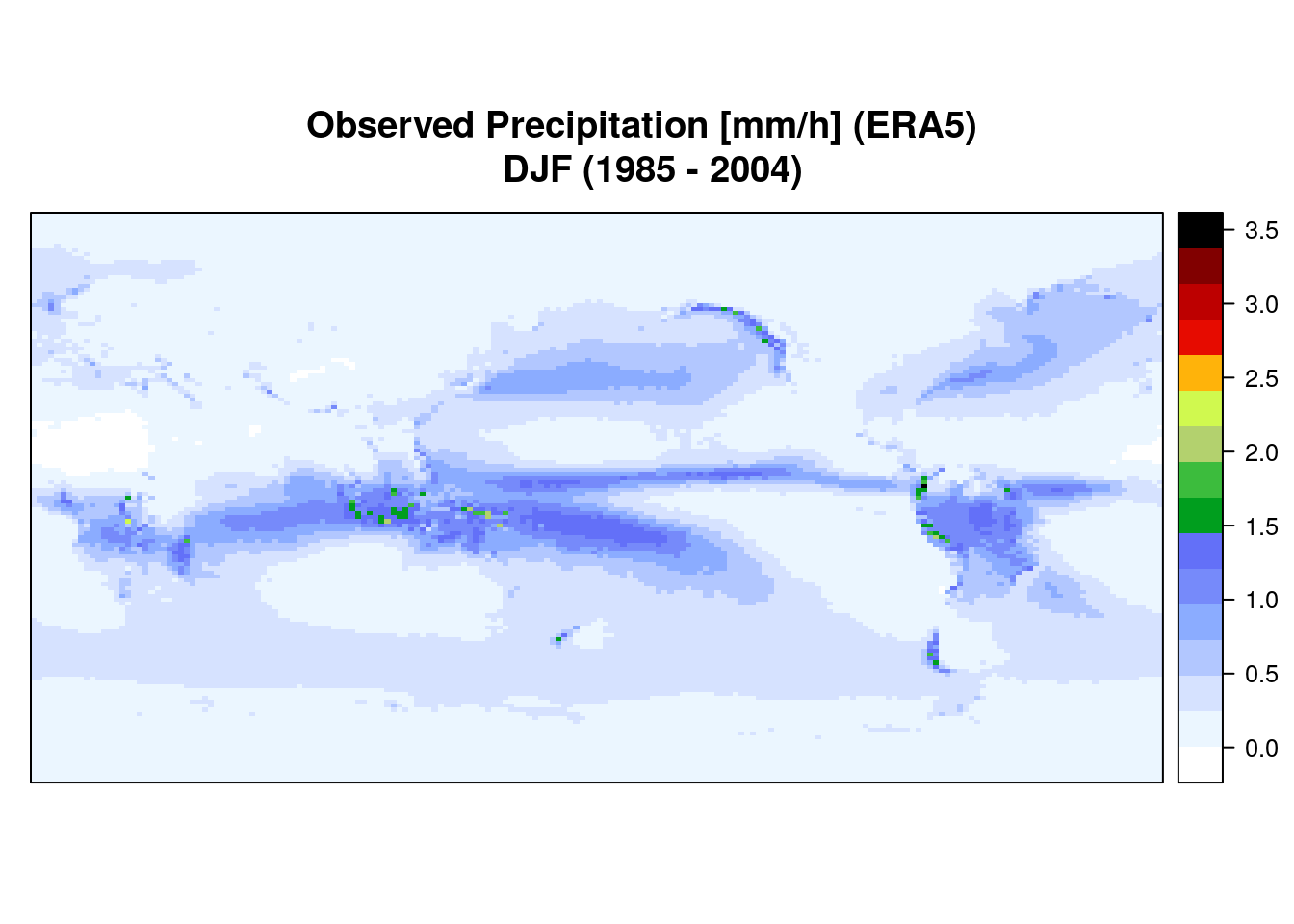
spplot(mean_pcp_historical,
            main = "Simulated precipitation [mm/h] (HadGEM2-ES) \n DJF (1985 - 2004)",
            col.regions = cpt("ncl_precip2_17lev"))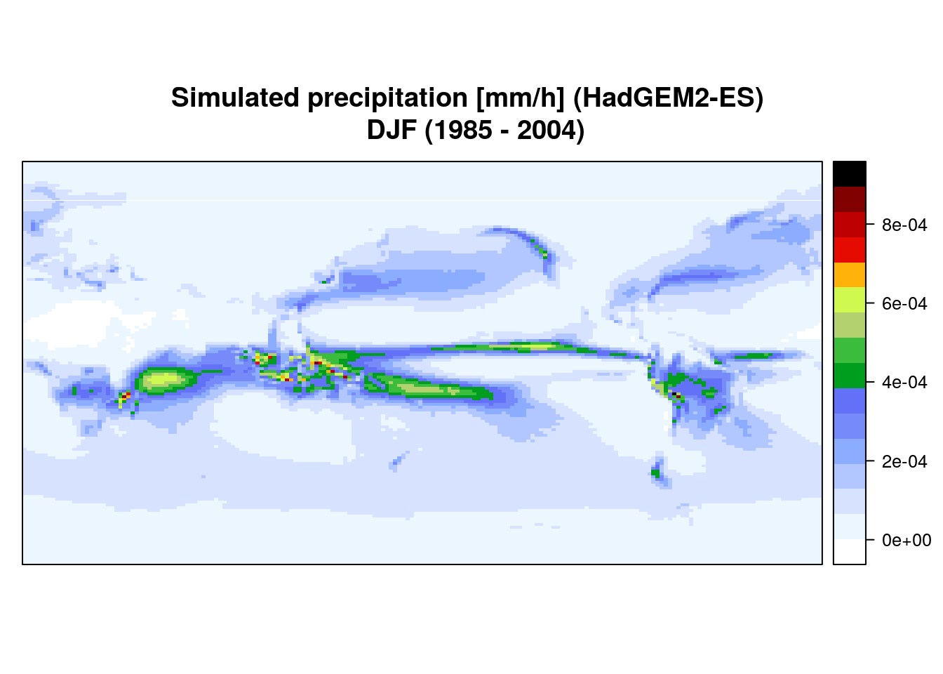
spplot(mean_pcp_historical - mean_pcp_era,
            main = "Simulated - Observed precipitation [mm/h] \n DJF (1985 - 2004)",
            col.regions = cpt("ncl_precip2_17lev", n = length(seq(-3.4, 3.4, 0.01))),
       at= seq(-3.4, 3.4, 0.01))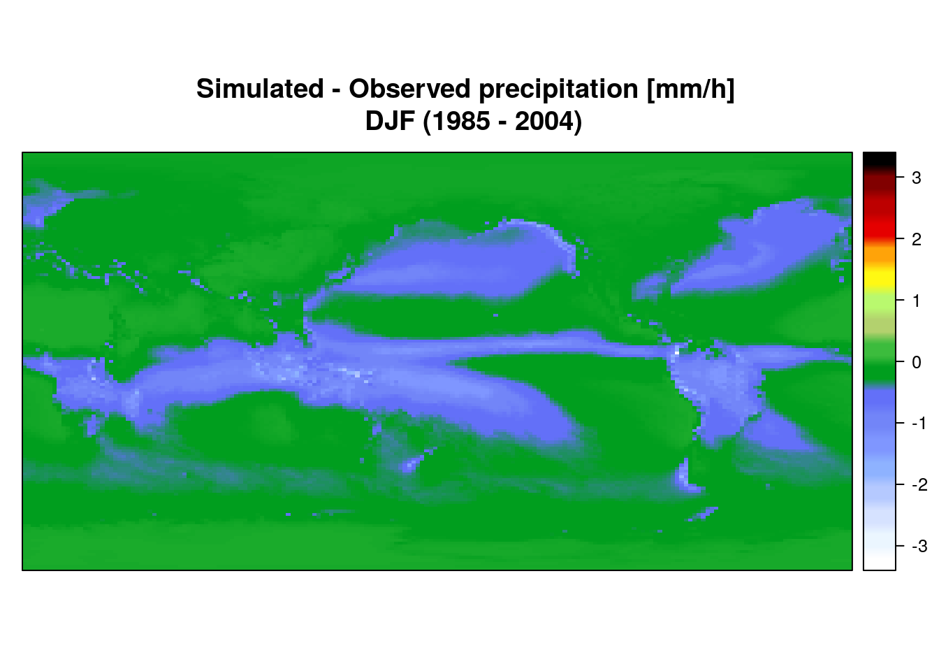
Ahora vamos a ver la temperatura
## class      : RasterBrick
## dimensions : 145, 192, 27840, 17  (nrow, ncol, ncell, nlayers)
## resolution : 1.875, 1.25  (x, y)
## extent     : -0.9375, 359.0625, -90.625, 90.625  (xmin, xmax, ymin, ymax)
## crs        : +proj=longlat +datum=WGS84 +ellps=WGS84 +towgs84=0,0,0
## source     : /home/sergio/Documents/UBA/dados/r_ERA5_t2m_DJF_1985-2004.nc
## names      : X1986.01.01.01.06.28, X1987.01.01.01.06.28, X1988.01.01.01.06.28, X1989.01.01.01.06.28, X1990.01.01.01.06.28, X1991.01.01.01.06.28, X1992.01.01.01.06.28, X1993.01.01.01.06.28, X1994.01.01.01.06.28, X1995.01.01.01.06.28, X1996.01.01.01.06.28, X1997.01.01.01.06.28, X1998.01.01.01.06.28, X1999.01.01.01.06.28, X2000.01.01.01.06.28, ...
## Date/time  : 1986-01-01 01:06:28, 2004-01-01 01:06:28 (min, max)
## varname    : t2m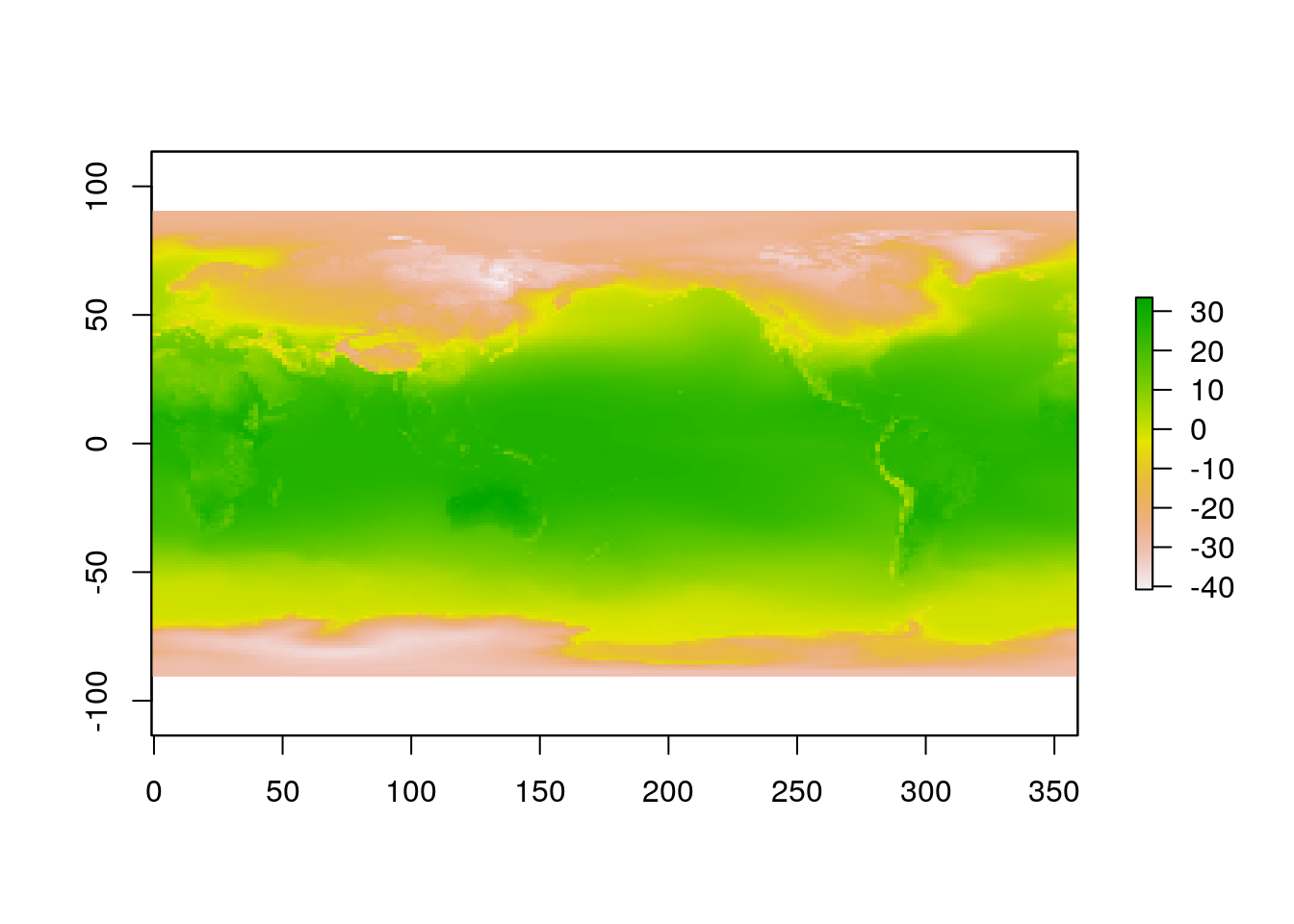
mean_t2m_era <- mean(t2m_era5 -273.15)

t2m_historical <- brick("dados/tas_Amon_HadGEM2-ES_historical_r1i1p1_DJF_1985-2004.nc")
plot(t2m_historical[[1]] - 273.15)
mean_t2m_historical <- mean(t2m_historical - 273.15)

spplot(mean_t2m_era,
            main = "Observed temperature at 2m [ºC] (ERA5) \n DJF (1985 - 2004)",
            at = seq(-40, 40, 1),
            col.regions = cpt("ncl_temp_diff_18lev"))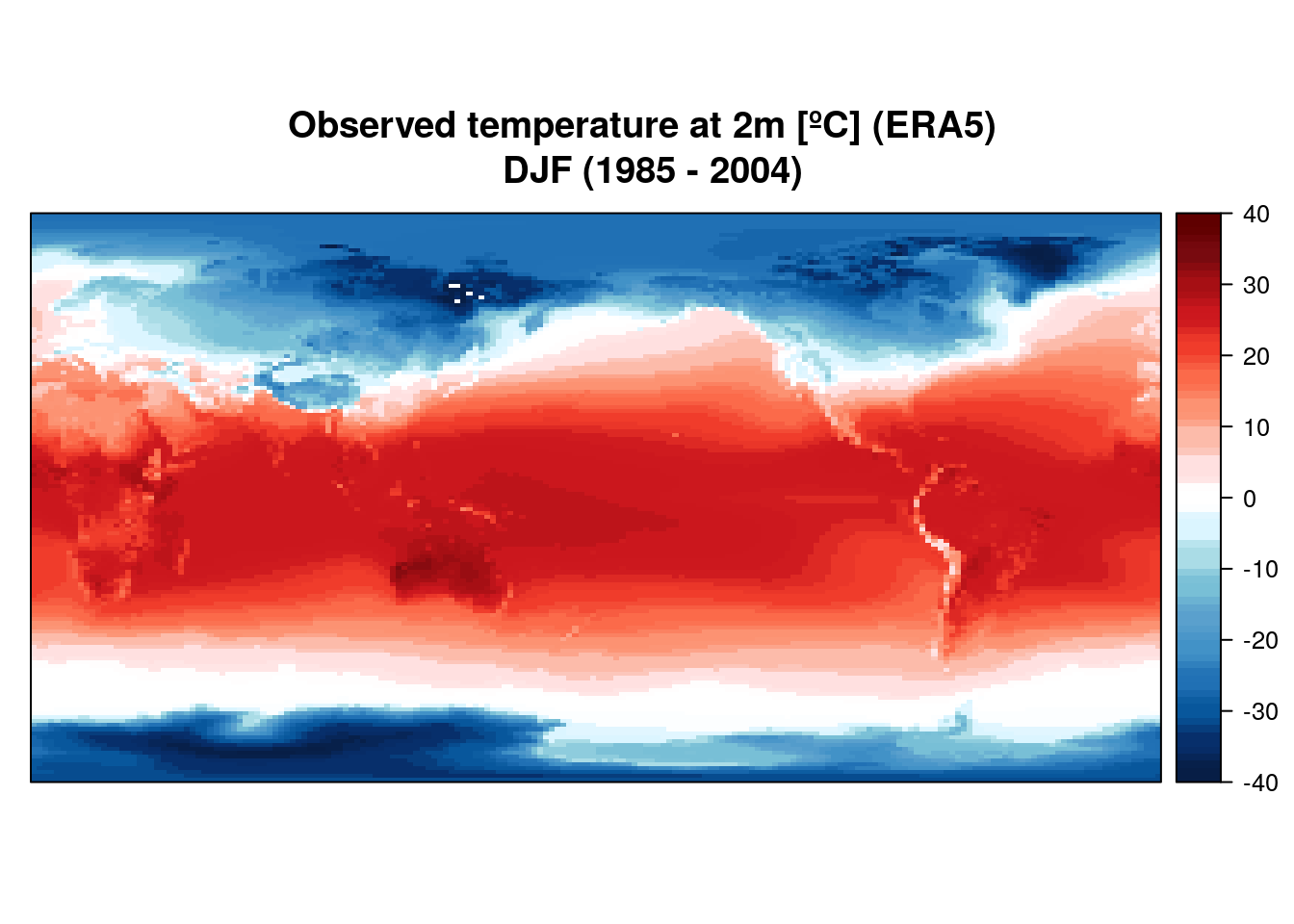
spplot(mean_t2m_historical,
            main = "Simulated temperature at 2m [ºC] (HadGEM2-ES) \n DJF (1985 - 2004)",
            at = seq(-40, 40, 1),
            col.regions = cpt("arendal_temperature"))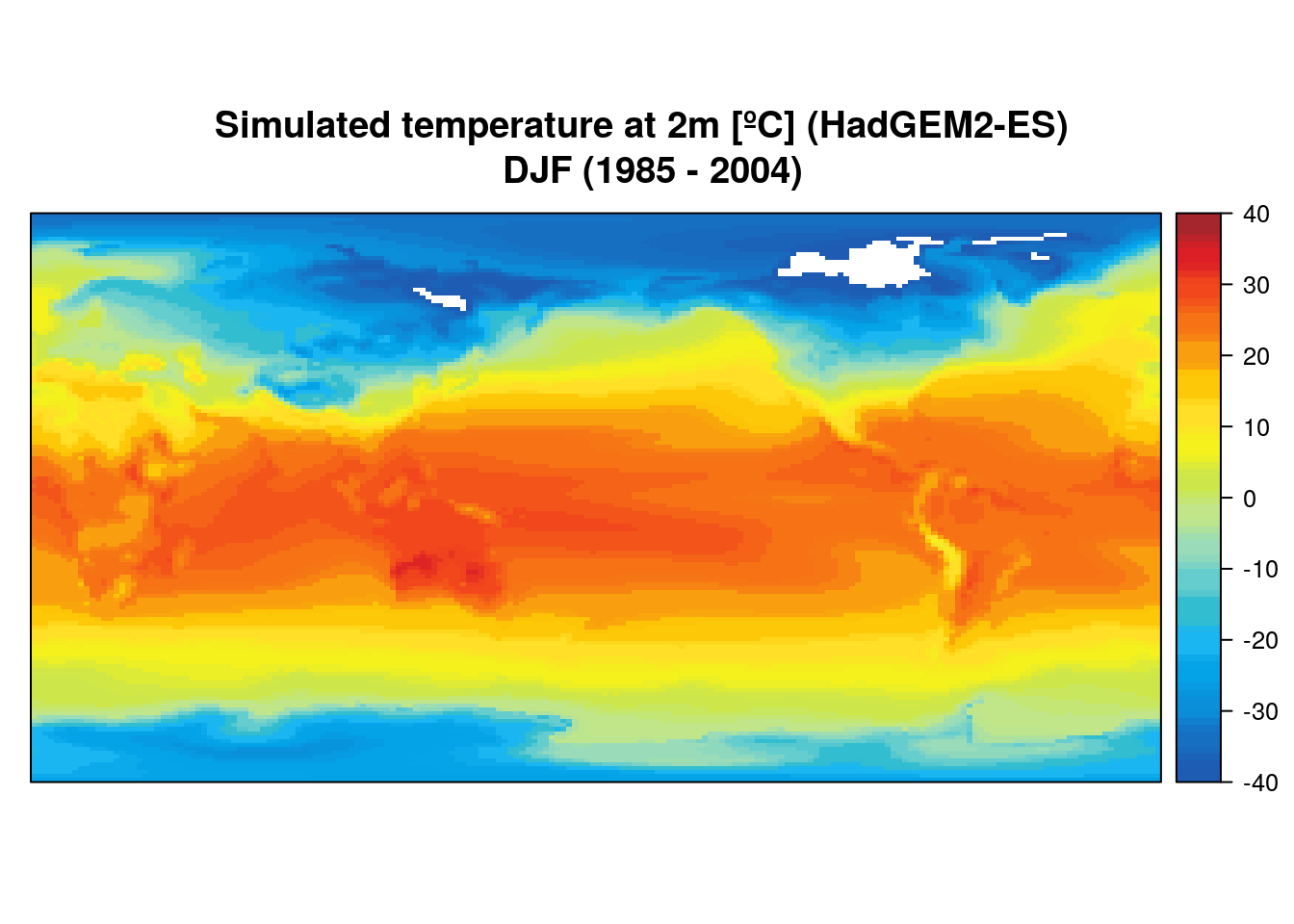
# Calculate the bias (how model is different from the observation):
pcp_bias <- (mean_pcp_historical - mean_pcp_era)
t2m_bias <- (mean_t2m_historical - mean_t2m_era)


spplot(pcp_bias,
            main = "Precipitation bias [mm/h] \n DJF (1985 - 2004)",
            at = seq(-3, 3, 0.1),
            col.regions = cpt("ncl_precip_diff_12lev"))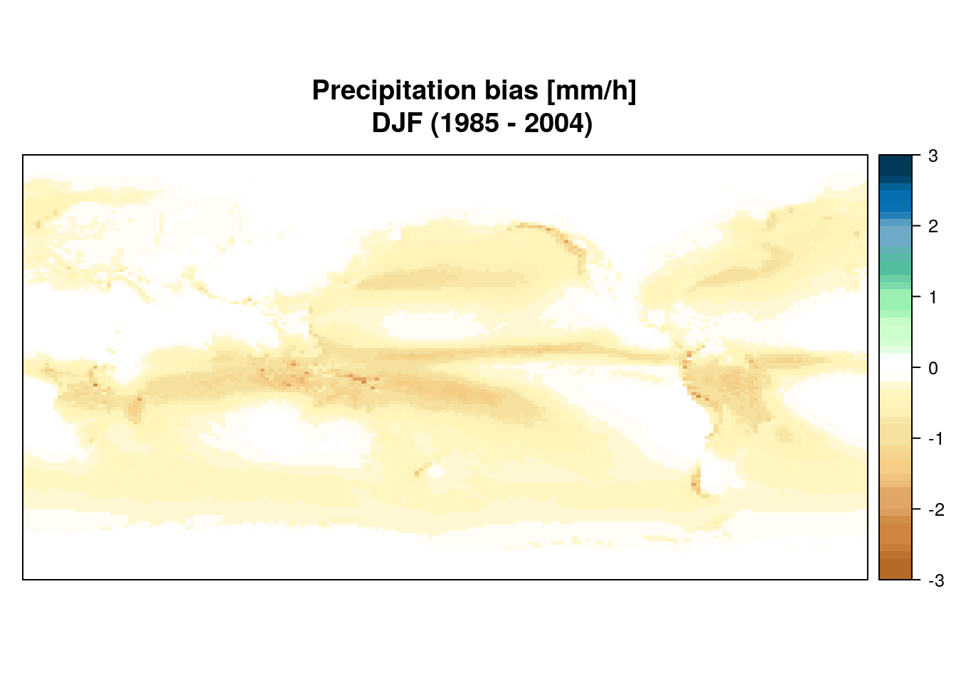
spplot(t2m_bias,
            main = "Temperature bias [ºC] \n DJF (1985 - 2004)",
            at = seq(-15, 15, 1),
            col.regions = cpt("ncl_temp_diff_18lev"))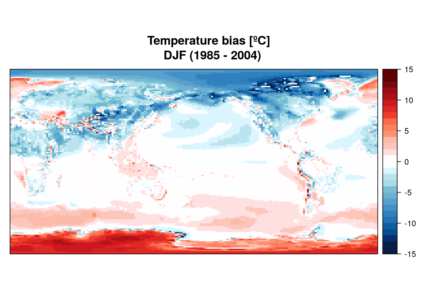
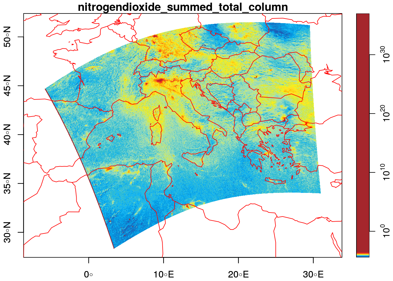
Y ahora vamos a ver como plotear datos de satelite de Sentinel 5P
library(stars)
(s5p = system.file("sentinel5p/S5P_NRTI_L2__NO2____20180717T120113_20180717T120613_03932_01_010002_20180717T125231.nc", package = "starsdata"))
## [1] "/home/sergio/R/x86_64-pc-linux-gnu-library/3.6/starsdata/sentinel5p/S5P_NRTI_L2__NO2____20180717T120113_20180717T120613_03932_01_010002_20180717T125231.nc"nit.c = read_stars(s5p, sub = "//PRODUCT/SUPPORT_DATA/DETAILED_RESULTS/nitrogendioxide_summed_total_column",
curvilinear = c("//PRODUCT/longitude",
"//PRODUCT/latitude"),
driver = NULL)## //PRODUCT/longitude,
## //PRODUCT/latitude,
## //PRODUCT/SUPPORT_DATA/DETAILED_RESULTS/nitrogendioxide_summed_total_column,Y el plot es
plot(nit.c,
     breaks = "hclust",
     reset = FALSE,
     axes = TRUE,
     logz = TRUE,
     key.length = 1,
     col = cpt("arendal_temperature"))
maps::map('world', add = TRUE, col = 'red')