Chapter 5 Emission Factors

An emission factor is the amount of mass of pollutant generated by activities (Pulles and Heslinga 2010). In the case of vehicles, the emission factor is the mass of pollutant per traveled distance \(g \cdot km^{-1}\) in metric units. The distance unit could be different, like miles for instance. The type of groups depends on the measurement used when developing the emission factors.

There are hot and cold exhaust emissions. Hot exhaust emissions are produced by a vehicle when its engine and exhaust after-treatment system are at their normal operating temperatures and Cold during the vehicle warm-up phase (P et al. 2009).

The emission factors come from measurements of pollutants emitted by the sources. In the case of vehicles, the dynamometer measurements of the emission factors are the mass of pollutant collected during the distance traveled by a vehicle following a specific driving cycle. The Federal Test Procedure (FTP) is a test to certify the vehicle emissions under the driving cycles such as FTP-75. This driving cycle has a duration of 1874 \(s\) for a distance of 17783 \(m\) and an average speed of 34.12 \(km \cdot h^{-1}\) (Barlow 2009).

In the literature, it is possible to find the different type of emission factors. For instance, in Europe, during the development of the project Assesment of Reliability of Transport Emission Models and Inventory Systems (ARTEMIS), the traffic situation model was developed. The model concept consists in the combination of parameters that affects vehicle kinematics and engine operation: type of road, sinuosity and gradient, traffic conditions or level of service (free-flow, heavy, saturated and stop and go) and average speed by the speed limit of the road (Boulter and Barlow 2009). Measurements of vehicular emissions under each traffic situation lead to emission factors by traffic situation, used in the Handbook of Emission Factors (HBEFA, www.hbefa.net).

There is another approach based on a 1 Hz measurement of emissions, where the pollutants are measured on real live traffic driving. Emission factors can be derived here using mainly two approaches. One approach is applying the Vehicular Specific Power (VSP) (Jimenez et al. 1999). This method is used in the Motor Vehicle Emission Simulator (MOVES) (Koupal et al. 2003) and the International Vehicle Emissions model (IVE) (Davis et al. 2005). Another approach is to apply the Passenger car, and Heavy-duty Emission Model (PHEM), which is based on instantaneous engine power demand and engine speed developed during the ARTEMIS project (Barlow 2009, Boulter and Barlow (2009)).

Perhaps the most used approach to obtain emission factors are speed functions. As emissions tests on driving cycles are valid for only one average speed, measuring emissions of different driving cycles at different average speeds, allows obtaining point clouds where regression is applied, obtaining an emission factor as a speed function. The literature shows experiments in different parts of the world, such as in Chile (Corvalán, Osses, and Urrutia 2002) and Europe (Ntziachristos and Samaras 2000). However, probably the most used source of emission factors as speed functions are the European emission guidelines developed by the European Monitoring and Evaluation Programme (EMEP, http://www.emep.int/) and published by the European Environment Agency (EEA, https://www.eea.europa.eu/themes/air/emep-eea-air-pollutant-emission-inventory-guidebook/emep) (Ntziachristos and Samaras 2016), which are included in the VEIN model.

Another aspect important in vehicular emissions is the degradation of the emissions of old vehicles. Over time, the different part of the cars suffers deterioration, increasing the emissions. Therefore, approaches have been developed to account for this effect in inventories. One method consists in determining functions that increment the emissions by accumulated mileage, such as studies of Corvalán and Vargas (2003).

In Brazil, the emission factors are reported by the Environmental Protection Agency of São Paulo CETESB (2015), in their vehicular emissions inventory report. Light vehicles emission factors come from average measurements of the FTP75 driving cycle, and motorcycle emission factors come from average measurements of World Motorcycle Test Cycle (WMTC) and HDV from the European Stationary Cycle (ETC).

I developed the VEIN model in Brazil, but users of other parts of the world may be interested in using the model, the approach in VEIN has to allow flexibility to the user. Therefore, the emission factors approach in VEIN consists of three options, as shown in Fig. (5.1). The first approach consists of local emissions factors by the age of use, such as the one from CETESB (2015), denoted as local_ef in the green circle. The second approach consisted in selecting speed functions from Ntziachristos and Samaras (2016), available in VEIN and denoted as the grey box as speed_ef. The third approach consists in incorporating speed variation from the speed function into the local emission factors by the age of use. In any case, VEIN uses a function to account for the degradation of emissions due to accumulated mileage (denoted in a grey box as emis_det). These emissions are inputted into the emission estimation function.

The following sections show how to do this calculation in VEIN, step by step.

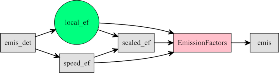
Figure 5.1: Structuring an emissions inventories with VEIN

5.1 Speed functions ef_ldv_speed and ef_hdv_speed

The estimation of emissions in VEIn is shown the equation (5.1):

\[\begin{equation} EH_{i,j,k,l,m} =F_{i,j,k,l} \cdot L_i \cdot EF(V_{i,l})_{j,k,m} \cdot DF_{j,k} \tag{5.1} \end{equation}\]

where \(EH_{i,j,k,l,m}\) is the emission for each street link \(i\), vehicle category from composition \(k\), hour \(l\) and pollutant \(m\), \(F_{i,j,k,l}\) is the vehicular flow calculated in Eq. 1. \(L_i\) is the length of the street link \(i\). \(EF(V_{i,l})_{j,k,m}\) is the emission factor of each pollutant \(m\). \(DF_{j,k}\) is the deterioration factor for vehicle of type \(j\) and age of use \(k\), explained in detail in section 5.5.

These functions return speed functions as \(f(V)\). The functions come from the EMEP/EEA emissions guidelines (Ntziachristos and Samaras 2016) and are available in PDF reports. The equations and their parameters were translated to a spreadsheet and loaded internally in VEIN. Therefore, the user only must enter the required parameters obtaining the desired function. The functions respect the assumptions and speed limits.

5.1.1 Emission factors of LDV depending on the speed with the function ef_ldv_speed

The arguments for ef_ldv_speed are:

args(ef_ldv_speed)

## function (v, t = "4S", cc, f, eu, p, x, k = 1, 
## show.equation = FALSE) 

• v: Category of vehicle: “PC”, “LCV”, “Motorcycle” or “Moped”.
• t: Sub-category of vehicle: PC: “ECE_1501”, “ECE_1502”, “ECE_1503”, “ECE_1504” , “IMPROVED_CONVENTIONAL”, “OPEN_LOOP”, “ALL”, “2S” or “4S”. LCV: “4S”, Motorcycle: “2S” or “4S”. Moped: “2S” or “4S”.
• cc: Size of engine in cc: PC: “<=1400”, “>1400”, “1400_2000”, “>2000”, “<=800”, “<=2000”. Motorcycle: “>=50” (for “2S”), “<=250”, “250_750”, “>=750”. Moped: “<=50”. LCV : “<3.5” for gross weight.
• f: Type of fuel: “G”, “D”, “LPG” or “FH” (Full Hybrid: starts by electric motor).
• eu: Euro standard: “PRE”, “I”, “II”, “III”, “III+DPF”, “IV”, “V”, “VI” or “VIc”.
• p: Pollutants: Criteria: “CO”, “NOx”, “HC”, “PM”, “CH4”, “NMHC”, “CO2”, “SO2”, “Pb”, “FC” (Fuel Consumption).
• PAH and POP: “indeno(1,2,3-cd)pyrene”, “benzo(k)fluoranthene”, “benzo(b)fluoranthene”, “benzo(ghi)perylene”, “fluoranthene”, “benzo(a)pyrene”, “pyrene”, “perylene”, “anthanthrene”, “benzo(b)fluorene”, “benzo(e)pyrene”, “triphenylene”, “benzo(j)fluoranthene”, “dibenzo(a,j)anthacene”, “dibenzo(a,l)pyrene”, “3,6-dimethyl-phenanthrene”, “benzo(a)anthracene”, “acenaphthylene”, “acenapthene”, “fluorene”, “chrysene”, “phenanthrene”, “napthalene”, “anthracene”, “coronene”, “dibenzo(ah)anthracene” Dioxins and Furans: “PCDD”, “PCDF”, “PCB”.
• Metals: “As”, “Cd”, “Cr”, “Cu”, “Hg”, “Ni”, “Pb”, “Se”, “Zn”.
• NMHC:
• ALKANES: “ethane”, “propane”, “butane”, “isobutane”, “pentane”, “isopentane”, “hexane”, “heptane”, “octane”, “TWO_methylhexane”, “nonane”, “TWO_methylheptane”, “THREE_methylhexane”, “decane”, “THREE_methylheptane”, “alcanes_C10_C12”, “alkanes_C13”.
• CYCLOALKANES: “cycloalcanes”.
• ALKENES: “ethylene”, “propylene”, “propadiene”, “ONE_butene”, “isobutene”, “TWO_butene”, “ONE_3_butadiene”, “ONE_pentene”, “TWO_pentene”, “ONE_hexene”, “dimethylhexene”.
• ALKYNES:“ONE_butine”, “propine”, “acetylene”.
• ALDEHYDES: “formaldehyde”, “acetaldehyde”, “acrolein”, “benzaldehyde”, “crotonaldehyde”, “methacrolein”, “butyraldehyde”, “isobutanaldehyde”, “propionaldehyde”, “hexanal”, “i_valeraldehyde”, “valeraldehyde”, “o_tolualdehyde”, “m_tolualdehyde”, “p_tolualdehyde”.
• KETONES: “acetone”, “methylethlketone”.
• AROMATICS: “toluene”, “ethylbenzene”, “m_p_xylene”, “o_xylene”, “ONE_2_3_trimethylbenzene”, “ONE_2_4_trimethylbenzene”, “ONE_3_5_trimethylbenzene”, “styrene”, “benzene”, “C9”, “C10”, “C13”.
• k: Multiplication factor.
• show.equation: Option to see (or not) the equation parameters.

It is essential that the user enters the right values into the arguments because the final category must match. If the user enters values that do not match, the resulting speed function will be wrong. There are 146 matches. The probably most used combinations are:

Table 5.1: Most used combinations for emission factors for LDV

Argument	Value
v	PC LCV Motorcycles
t	4S
cc	<=1400 1400_2000 >2000
f	G D
eu	PRE I II III IV V VI
p	CO NOx HC FC PM

The returning speed function represents how a type of vehicle emits pollutants on average. The Fig. (5.2) shows the emissions of CO by Passenger Cars with technologies Pre Euro and Euro I from Ntziachristos and Samaras (2016). Higher emissions occurs at low average speeds and older vehicles with technologies pre Euro emit more than vehicles with Euro I. Even more, the average emissions of Pre Euro are 29.31 \(g \cdot km^{-1}\) and Euro I 2.61 \(g \cdot km^{-1}\), meaning that, on average, a vehicle Pre euro is 14 times higher than a vehicle with euro I.

The Fig. (5.2) shows the plot using the package ggplot2 (Wickham 2009). This package requires that the data must be in long format.

library(vein)
library(ggplot2)
ef1 <- ef_ldv_speed(v = "PC", cc = "<=1400", f = "G",
                    eu = "PRE", p = "CO", show.equation = F)
ef2 <- ef_ldv_speed(v = "PC", cc = "<=1400", f = "G",
                    eu = "I", p = "CO", show.equation = F)
V <- 0:110
df <- data.frame(EF = c(ef1(V), ef2(V)))
df$V = V
df$Euro <- factor(c(rep("PRE", 111), rep("I", 111)),
                  levels = c("PRE", "I"))
ggplot(df, aes(V, EF, colour = Euro)) + geom_point(size = 3) +
  geom_line() + theme_bw()+
  labs(y = "CO[g/km]", x = "[km/h]")

Figure 5.2: Emission factor as a speed function

5.1.2 Emission factors of HDV depending on the speed with the function ef_hdv_speed

The arguments for ef_hdv_speed are:

args(ef_hdv_speed)

## function (v, t, g, eu, x, gr = 0, l = 0.5, 
## p, k = 1, show.equation = FALSE) 

• v Category of vehicle: “Coach”, “Trucks” or “Ubus”
• t Sub-category of vehicle: “3Axes”, “Artic”, “Midi”, “RT,”Std" and “TT”
• g Gross weight of each category: “<=18”, “>18”, “<=15”, “>15 & <=18”, “<=7.5”, - “>7.5 & <=12”, “>12 & <=14”, “>14 & <=20”, “>20 & <=26”, “>26 & <=28”, “>28 & <=32”, “>32”, “>20 & <=28”, “>28 & <=34”, “>34 & <=40”, “>40 & <=50” or “>50 & <=60”
• `eu Euro emission standard: “PRE”, “I”, “II”, “III”, “IV” and “V”
• `gr Gradient or slope of road: -0.06, -0.04, -0.02, 0.00, 0.02. 0.04 or 0.06
• l Load of the vehicle: 0.0, 0.5 or 1.0
• p Pollutant: Criteria: “CO”, “NOx”, “HC”, “PM”, “CH4”, “NMHC”, “CO2”, “SO2”, “Pb”, “FC” (Fuel Consumption).
• PAH and POP: “indeno(1,2,3-cd)pyrene”, “benzo(k)fluoranthene”, “benzo(b)fluoranthene”, “benzo(ghi)perylene”, “fluoranthene”, “benzo(a)pyrene”, “pyrene”, “perylene”, “anthanthrene”, “benzo(b)fluorene”, “benzo(e)pyrene”, “triphenylene”, “benzo(j)fluoranthene”, “dibenzo(a,j)anthacene”, “dibenzo(a,l)pyrene”, “3,6-dimethyl-phenanthrene”, “benzo(a)anthracene”, “acenaphthylene”, “acenapthene”, “fluorene”, “chrysene”, “phenanthrene”, “napthalene”, “anthracene”, “coronene”, “dibenzo(ah)anthracene”
• Dioxins and Furans: “PCDD”, “PCDF”, “PCB”.
• Metals: “As”, “Cd”, “Cr”, “Cu”, “Hg”, “Ni”, “Pb”, “Se”, “Zn”.
• NMHC:
• ALKANES: “ethane”, “propane”, “butane”, “isobutane”, “pentane”, “isopentane”, “hexane”, “heptane”, “octane”, “TWO_methylhexane”, “nonane”, “TWO_methylheptane”, “THREE_methylhexane”, “decane”, “THREE_methylheptane”, “alcanes_C10_C12”, “alkanes_C13”.
• CYCLOALKANES: “cycloalcanes”.
• ALKENES: “ethylene”, “propylene”, “propadiene”, “ONE_butene”, “isobutene”, “TWO_butene”, “ONE_3_butadiene”, “ONE_pentene”, “TWO_pentene”, “ONE_hexene”, “dimethylhexene”.
• ALKYNES:“ONE_butine”, “propine”, “acetylene”.
• ALDEHYDES: “formaldehyde”, “acetaldehyde”, “acrolein”, “benzaldehyde”, “crotonaldehyde”, “methacrolein”, “butyraldehyde”, “isobutanaldehyde”, “propionaldehyde”, “hexanal”, “i_valeraldehyde”, “valeraldehyde”, “o_tolualdehyde”, “m_tolualdehyde”, “p_tolualdehyde”.
• KETONES: “acetone”, “methylethlketone”.
• AROMATICS: “toluene”, “ethylbenzene”, “m_p_xylene”, “o_xylene”, “ONE_2_3_trimethylbenzene”, “ONE_2_4_trimethylbenzene”, “ONE_3_5_trimethylbenzene”, “styrene”, “benzene”, “C9”, “C10”, “C13”.
• k: Multiplication factor.
• k Multiplication factor
• show.equation Option to see or not the equation parameters

V <- 0:130
ef1 <- ef_hdv_speed(v = "Trucks",t = "RT", g = "<=7.5",
                    e = "II", gr = 0,
l = 0.5, p = "HC", show.equation = FALSE)
ef2 <- ef_hdv_speed(v = "Trucks",t = "RT", g = "<=7.5",
                    e = "II", gr = 0.06,
l = 0.5, p = "HC", show.equation = FALSE)
plot(1:130, ef1(1:130), pch = 16, type = "b",
     ylab = "HC [g/km]", xlab = "Speed [km/h]")
lines(1:130, ef2(1:130), pch = 16, type = "b", col = "blue")

5.2 Local emission factors by age of use, EmissionFactors and EmissionFactorsList

The functions EmissionFactors and EmissionFactorsList create the classes with same names. The class EmissionFactors is also a data-frame with numeric columns with units of \(g \cdot km^{-1}\). This class is not used in critical steps of VEIN, and it has a purpose of creating a data-frame with numeric columns and units. The function is applied to a numeric vector, and it just converts it to units adding units to it.

In the case of EmissionFactorsList, this class is a list of functions \(f(V)\). This is useful because of the emis function, seen in detail on chapter 6, requires that the emission factors are functions of velocity \(f(V)\), regardless \(f(V)\) if it is constant or not. When this function is applied to a data-frame or a matrix, it returns a list, and each column of the data-frame or matrix is another list. Also, each row of the original data-frame is converted to a \(f(V)\).

The arguments or EmissionFactorsList and EmissionFactors are:

-x: Object with class “data.frame”, “matrix” or “numeric”

The following lines of code show examples using EmissionFactors. Firstly, we load the dataset of emission factors fe2015 for CO and the vehicles PC using gasoline PC_G and Light Trucks LT. The class of fe2015 is data-frame. The subset of the data is named DF_CO. The first six elements of the data-frame are numbers without units.

library(vein)
data(fe2015) #CETESB Emission factors
DF_CO <- fe2015[fe2015$Pollutant=="CO", c("PC_G", "LT")]
head(DF_CO)

##    PC_G    LT
## 1 0.171 0.027
## 2 0.216 0.012
## 3 0.237 0.012
## 4 0.273 0.005
## 5 0.275 0.379
## 6 0.204 0.416

The object EF_CO is of class EmissionFactors and “data-frame” and each observation has the units \(g \cdot km^{-1}\).

EF_CO <- EmissionFactors(DF_CO)
head(EF_CO)

## EmissionFactors:
##           PC_G           LT
## 1 0.171 [g/km] 0.027 [g/km]
## 2 0.216 [g/km] 0.012 [g/km]
## 3 0.237 [g/km] 0.012 [g/km]
## 4 0.273 [g/km] 0.005 [g/km]
## 5 0.275 [g/km] 0.379 [g/km]
## 6 0.204 [g/km] 0.416 [g/km]

class(EF_CO)

## [1] "EmissionFactors" "data.frame"

The plot of an object of class EmissionFactors shows a maximum nine emission factors. Fig. (5.3) shows the emission factors of both categories, where newer vehicles emit less and older vehicles emit more.

plot(EF_CO, xlab = "Age of use")

Figure 5.3: Emission factor of PC and LT by age of use

Regarding the class EmissionFactorsList, the print and summary methods are straightforward, only showing a description of the object. The example of the following lines of code also uses the same set of Emission Factors from CETESB (2015). The resulting object, EF_COL, is of class EmissionFactorsList and list. The print of the object shows only a description of the first and last member of the list object.

EFL_CO <- EmissionFactorsList(DF_CO)
class(EFL_CO)

## [1] "EmissionFactorsList" "data.frame"

EFL_CO

## This EmissionFactorsList has  2  lists
## First has  36  functions
## Last has  36  functions

Indeed, if we want to see the content of the EmissionFactorsList we have to extract the elements of the list. EFL_CO has two lists; one for PC and one for LT. Then, each list has 36 functions, the command class(EFL_CO[[1]][[1]]) shows the object is a function \(f(V)\).

EFL_CO[[1]][[1]]

## function(V) x[j,i]
## <bytecode: 0x55dd82d72d80>
## <environment: 0x55dd847abc50>

Also, as the speed functions are constant, there is no need to add values of V.

EFL_CO[[1]][[1]](100) # constant speed function

## [1] 0.171

EFL_CO[[1]][[1]](0)   # constant speed function

## [1] 0.171

Finally, after extracting the value, Fig. (5.4) shows the same figure as Fig. (5.3)

efco1 <- sapply(1:36, function(i) EFL_CO[[1]][[i]]())
efco2 <- sapply(1:36, function(i) EFL_CO[[2]][[i]]())
df <- EmissionFactors(cbind(efco1, efco2))
plot(df, xlab = "Age of use")

Figure 5.4: Emission factor of PC and LT

5.3 Incorporating speed variation with the functions ef_ldv_scaled and ef_hdv_scaled

The functions in section 5.1 and 5.2 showed the speed and local emission factors respectively. However, the user might have local and constant emission factors depending only on the age of use, but also, outputs from a traffic demand model which includes speed. Under those circumstances, it would be interesting to investigate the effects of the average rate of traffic flow. VEIN provides for functions to transform a constant emission factor by the age of use into a speed dependent function.

These functions are called ef_ldv_scaled and ef_hdv_scaled. The concept is explained in detail in my Ph.D. thesis (Ibarra-Espinosa 2017). The idea comes from revisiting the nature of the local emission factors. The Brazilian emission factors consist of average measurements for emissions certification tests which use the driving cycles Federal Test Procedure FTP-75 for LDV, World Motorcycle Test Cycle (WMTC) for motorcycles, and also the European Stationary Cycle (ESC) for HDV (CETESB 2015). The average speed of FTP-75 and WMTC are known, being 34.2 \(km \cdot h^{-1}\) and 54.7 \(km \cdot h^{-1}\) based on the reference report on driving cycles from the Transport and Research Laboratory (TRL) (Barlow 2009). In the case of ESC, the user might search on literature a way to relate this cycle with an average speed.

Coming back to the CETESB (2015) emission factors, these are annual average values of emissions for the different technologies to accomplish Brazilian emission standards, which are valid only for a specific average speed. If two vehicles have similar technology but different emission factors, one constant and other speed function, it would be possible to relate them. These functions use the speed to relate both emission factors. The condition to transform a constant emission factor into a speed dependent function is that the new speed-dependent function must be of the same value at the speed which is representative for the local factor, And the values at other speeds are the incorporation of the speed variation. The equation (5.2) shows the procedure:

\[\begin{equation} EF_{scaled}(V_{i,l})_{j,k,m}=EF(V_{i,l})_{j,k,m} \cdot \frac{EFlocal_{j,k,m}}{{EF(Vdc_{i,l})_{j,k,m}}} \tag{5.2} \end{equation}\]

Where \(EF_{scaled}(V_{i,l})_{j,k,m}\) is the scaled emission factor and \(EF(V_{i,l})_{j,k,m}\) is the Copert emission factor for each street link \(i\), vehicle from composition \(k\), hour \(l\) and pollutant \(m\). \(EFlocal_{j,k,m}\) represents the constant emission factor (not as speed functions). \(EF(Vdc_{i,l})_{j,k,m}\) are Copert emission factors with average speed value of the respective driving cycle for the vehicular category \(j\).

The functions ef_ldv_scaled and ef_hdv_scaled return scaled emissions factors automatically. The arguments are:

args(ef_ldv_scaled)

## function (df, dfcol, SDC = 34.12, v, t = "4S", cc, f, eu, p) 
## NULL

• df: Data-frame with emission factors (Deprecated in 0.3.10).
• dfcol: Numeric vector with the emission factors constant by age of use. These emission factors are the target to incorporate speed variation.
• SDC: A number with the speed of the driving cycle of the emission factors from the argument dfcol. The resulting speed functions will return the same values of dfcol at the speed SDC. The default is 34.12 “km/h”.
• v. Category of vehicle: “PC”, “LCV”, “Motorcycle” or “Moped”.
• t. Character; sub-category of vehicle: PC: “ECE_1501”, “ECE_1502”, “ECE_1503”, “ECE_1504” , “IMPROVED_CONVENTIONAL”, “OPEN_LOOP”, “ALL”, “2S” or “4S”. LCV: “4S”, Motorcycle: “2S” or “4S”. Moped: “2S” or “4S”. The default is 4S.
• cc. Character; size of engine in cc: PC: “<=1400”, “>1400”, “1400_2000”, “>2000”, “<=800”, “<=2000”. Motorcycle: “>=50” (for “2S”), “<=250”, “250_750”, “>=750”. Moped: “<=50”. LCV : “<3.5” for gross weight.
• f: Character; type of fuel: “G”, “D”, “LPG” or “FH” (Full Hybrid: starts by electric motor).
• eu: Character; euro standard: “PRE”, “I”, “II”, “III”, “III+DPF”, “IV”, “V”, “VI” or “VIc”.
• p: Character; pollutant: “CO”, “FC”, “NOx”, “HC” or “PM”.

And the argument of ef_hdv_scaled are:

args(ef_hdv_scaled)

## function (df, dfcol, SDC = 34.12, v, t, g, eu, gr = 0, l = 0.5, 
##     p) 
## NULL

• df: Data-frame with emission factors (Deprecated in 0.3.10).
• dfcol: Numeric vector with the emission factors constant by age of use. - SDC Speed of the driving cycle.
• v: Category vehicle: “Coach”, “Trucks” or “Ubus”
• t: Sub-category of of vehicle: “3Axes”, “Artic”, “Midi”, “RT,”Std" and “TT”
• g: Gross weight of each category: “<=18”, “>18”, “<=15”, “>15 & <=18”, “<=7.5”, “>7.5 & <=12”, “>12 & <=14”, “>14 & <=20”, “>20 & <=26”, “>26 & <=28”, “>28 & <=32”, “>32”, “>20 & <=28”, “>28 & <=34”, “>34 & <=40”, “>40 & <=50” or “>50 & <=60”
• eu: Euro emission standard: “PRE”, “I”, “II”, “III”, “IV” and “V”
• gr: Gradient or slope of road: -0.06, -0.04, -0.02, 0.00, 0.02. 0.04 or 0.06
• l: Load of the vehicle: 0.0, 0.5 or 1.0
• p: Pollutant: “CO”, “FC”, “NOx” or “HC”

5.4 Cold Starts

Cold start emissions are produced during engine startup when the engine and catalytic converter system has not reached its normal operating temperature. Several studies have shown a significant impact on these types of emissions (Chen et al. 2011, Weilenmann, Favez, and Alvarez (2009)). Under this condition emissions will be higher, and if the atmospheric temperature decreases, cold start emissions will increase regardless of whether the catalyst has reached its optimum temperature for functioning (Boulter and Barlow 2009). VEIN also considers cold start emissions using the approach outlined in Copert (Ntziachristos and Samaras 2016), as shown in equation (5.3).

\[\begin{equation} EC_{i,j,k,l,m} =\beta_{j} \cdot F_{i,j,k,l} \cdot L_i \cdot EF(V_{i,l})_{j,k,m} \cdot DF_{j.k} \cdot \left(EF_{\mbox{cold}}(ta_n,V_{i,l})_{j,k,m}-1\right) \tag{5.3} \end{equation}\]

This approach adds two terms to Eq. . The first term \(EF_{cold}(ta_n,V_{i,l})_{j,k,m}-1\) is the emission factors for cold start conditions at each street link \(i\), vehicle category from composition \(k\), hour \(l\) and pollutant \(m\) and monthly average temperature \(n\). (Ntziachristos and Samaras 2016) suggest using monthly average temperature.

The second term \(\beta_j\) is the fraction of mileage driven with a cold engine/catalyst (Ntziachristos and Samaras 2016). The VEIN model incorporates a dataset of cold starts recorded during the implementation of the International Vehicle Emissions (IVE) model (Davis et al. 2005) in São Paulo (Lents et al. 2004), which provides the hourly mileage driven with cold start conditions.

The function for cold start emission factors is ef_ldv_cold and its arguments are:

args(ef_ldv_cold)

## function (v = "LDV", ta, cc, f, eu, p, k = 1, 
## show.equation = FALSE) 

where:

• v: Category of vehicle: “LDV”.
• ta: Ambient temperature. Monthly mean can be used.
• cc: Size of engine in cc: “<=1400”, “1400_2000” or “>2000”.
• f: Type of fuel: “G”, “D” or “LPG”.
• eu: Euro standard: “PRE”, “I”, “II”, “III”, “IV”, “V”, “VI” or “VIc”.
• p: Pollutant: “CO”, “FC”, “NOx”, “HC” or “PM”.
• k: Multiplication factor.
• show.equation: Option to see or not the equation parameters.

ef1 <- ef_ldv_cold(ta = -5, cc = "<=1400", 
                   f ="G", eu = "I", p = "CO")
ef2 <- ef_ldv_cold(ta = 0, cc = "<=1400", 
                   f ="G", eu = "I", p = "CO")
ef3 <- ef_ldv_cold(ta = 5, cc = "<=1400", 
                   f ="G", eu = "I", p = "CO")
ef4 <- ef_ldv_cold(ta = 10, cc = "<=1400", 
                   f ="G", eu = "I", p = "CO")

Figure 5.5: Cold Emission factor of PC CO (g/km)

There is another function called ef_ldv_cold_list which will be deprecated soon.

5.5 Deterioration

By default, VEIN includes deterioration factors from Copert (Ntziachristos and Samaras 2016). However, it is possible to include other sources, such as from (Corvalán and Vargas 2003) or includes deteriorated local emission factors, which covered with the function emis_det. This function returns deteriorated factors, as numeric vectors, multiplied with the emission factors of vehicles with 0 mileage.

The arguments of this functions are:

args(emis_det)

## function (po, cc, eu, km) 
## NULL

where:

• p: Pollutant.
• cc: Size of an engine in cc.
• eu: Euro standard: “PRE”, “I”, “II”, “III”, “III”, “IV”, “V”, “VI”.
• km: mileage in km. VEIN includes a dataset of mileage function named “fkm”.

data(fe2015)
data(fkm)
pckma <- cumsum(fkm$KM_PC_E25(1:24)) #vehicles with catalizer
x1 <- fe2015[fe2015$Pollutant == "CO", ]
x1E3 <- subset(x1, x1$Euro_LDV %in% c("III", "IV", "V"))$PC_G
x1E1 <- subset(x1, x1$Euro_LDV %in% c("I", "II"))$PC_G
det_E3 <- emis_det(po = "CO", cc = 1000, eu = "III",
                   km = pckma[1:length(x1E3)])
det_E1 <- emis_det(po = "CO", cc = 1000, eu = "III",
                   km = pckma[(length(x1E3) + 1):23 ])
original_EF <- x1$PC
deteriorated_EF <- x1$PC * c(det_E3, det_E1, rep(1, 13))
plot(x = 1:36, y = original_EF, type = "b", pch = 15, 
     col = "blue",
     ylab = "CO[g/km]", xlab = "Age of use")
lines(x = 1:36, y = deteriorated_EF,  type = "b", pch = 16, 
      col = "red")

Figure 5.6: Deteriorated (red) and not-deteriorated (blue) EF CO

5.6 Evaporative emissions ef_evap

Evaporative emissions are essential sources of hydrocarbons, and these emissions are produced by vaporization of fuel due to variations in ambient temperatures (Mellios and Ntziachristos 2016, Andrade et al. (2017)). There are three types of emissions: diurnal emissions, due to increases in atmospheric temperature, which lead to the thermal expansion of vapor fuel inside the tank; running losses, when the fuel evaporates inside the tank due to the normal operation of the vehicle; and hot soak emissions, which occur when the hot engine is turned off. These methods implemented in VEIN were sourced from the evaporative emissions methods of Copert Tier 2 (Mellios and Ntziachristos 2016). In VEIN it is also possible to use local emission factors. Here I’m showing both approaches:

1. Tier 2 copert approach

\[\begin{equation} EV_{j,k} =\sum_{s}D_{s} \cdot \sum_{j}F_{j} \cdot (HS_{j,k}+de_{j,k}+RL_{j,k}) \tag{5.4} \end{equation}\]

where \(EV_{j}\) are the volatile organic compounds (VOC) evaporative emissions due to each type of vehicle \(j\). \(D_s\) is the “seasonal days” or number of days when the mean monthly temperature is within a determined range: [-5\(^{\circ}\),10\(^{\circ}\)C], [0\(^{\circ}\), 15\(^{\circ}\)C], [10\(^{\circ}\), 25\(^{\circ}\)C] and [20\(^{\circ}\), 35\(^{\circ}\)C]. \(F_{j,k}\) is the number of vehicles according to the same type \(j\) and age of use \(k\). \(HS_{j,k}\), \(de_{j,k}\) and \(RL_{j,k}\) are average hot/warm soak, diurnal and running losses evaporative emissions (\(\mathrm{g \cdot day^{-1}}\)), respectively, according to the vehicle type \(j\) and age of use \(k\). \(HS_{j,k}\) and \(RL_{j,k}\) are obtained using equations also sourced from (Mellios and Ntziachristos 2016):

\[\begin{equation} HS_{j,k} = x_{j,k} \cdot (c \cdot (p \cdot e_{shc}+(1-p) \cdot e_{swc})+(1-c) \cdot e_{shfi} ) \tag{5.5} \end{equation}\]

where: \(x\) is the number of trips per day for the vehicular type \(j\) and age of use \(k\). \(c\) is the fraction of vehicles with fuel return systems. \(p\) is the fraction of trips finished with a hot engine, for example, an engine that has reached its normal operating temperature and the catalyst has reached its light-off temperature (Ntziachristos and Samaras 2016). The light-off temperature is the temperature at the point when catalytic reactions occur inside a catalytic converter. \(e_{shc}\) and \(e_{swc}\) are average hot-soak and warm-soak emission factors for gasoline vehicles with carburettor or fuel return systems (\(\mathrm{g \cdot parking^{-1}}\)). \(e_{shfi}\) is the average hot-soak emission factors for gasoline vehicles equipped with fuel injection and non-return fuel systems (\(\mathrm{g \cdot parking^{-1}}\)).

The Eq. (5.6) shows the procedure.

\[\begin{equation} RL_{j,k} = x_{j,k} \cdot (c \cdot (p \cdot e_{rhc}+(1-p) \cdot e_{rwc})+(1-c) \cdot e_{rhfi} ) \tag{5.6} \end{equation}\]

where: \(x\) and \(p\) have the same meanings of Eq. (5.5). \(e_{rhc}\) and \(e_{rwc}\) are average hot and warm running losses emission factors for gasoline vehicles with carburettor or fuel return systems (\(\mathrm{g \cdot trip^{-1}}\)) \(e_{rhfi}\) are average hot running losses emission factors for gasoline vehicles equipped withfuel injection and non-return fuel systems (\(\mathrm{g \cdot trip^{-1}}\)).

It is recommended to estimate the number of trips per day (Mellios and Ntziachristos 2016), \(x\), as the division between the mileage and 365 times the length of trip: \(x = \frac{mileage_j}{(365 \cdot ltrip)}\).

However, the mileage of a vehicle is not constant throughout the years. Therefore, VEIN incorporates a dataset of equations to estimate mileage of different types of cars by the age of use (Bruni and Bales 2013).

The function for evaporative emission factors is ef_evap and it arguments are :

args(ef_evap)

## function (ef, v, cc, dt, ca, k = 1, show = FALSE) 
## NULL

where: - ef: Name of evaporative emission factor as eshotc (\(g \cdot proced^-1\)): mean hot-soak with carburator, eswarmc (\(g \cdot proced^-1\)): mean cold and warm-soak with carburator, eshotfi: mean hot-soak with fuel injection, erhotc (\(g \cdot trip^-1\)): mean hot running losses with carburator, erwarmc (\(g \cdot trip^-1\)) mean cold and warm running losses, erhotfi (\(g \cdot trip^-1\)) mean hot running losses with fuel injection. - v: Type of vehicles, “PC”, “Motorcycles”, “Motorcycles_2S” and “Moped” - cc: Size of engine in cc. PC “<=1400”, “1400_2000” and “2000” Motorcycles_2S: “<=50”. Motorcyces: “>50”, “<250”, “250_750” and “>750” - dt: Average daily temperature variation: “-5_10”, “0_15”, “10_25” and “20_35” - ca: Size of canister: “no” meaning no canister, “small”, “medium” and “large” - k: multiplication factor - show: when TRUE shows row of table with respective emission factor.

Example:

library(vein)
library(ggplot2)
library(cptcity)
dt <- c("-5_10", "0_15", "10_25", "20_35")
ef <- sapply(1:4, function(i){
  ef_evap(ef = "erhotc",v = "PC", cc = "<=1400",
                dt = dt[i], ca = "no",
                show = TRUE)
})

##        ef  units veh     cc    dt canister    g
## 28 erhotc g/trip  PC <=1400 -5_10       no 1.67
##        ef  units veh     cc   dt canister    g
## 21 erhotc g/trip  PC <=1400 0_15       no 2.39
##        ef  units veh     cc    dt canister    g
## 14 erhotc g/trip  PC <=1400 10_25       no 3.25
##       ef  units veh     cc    dt canister    g
## 7 erhotc g/trip  PC <=1400 20_35       no 5.42

df <- data.frame(ef = ef, temp = c(0, 10, 20, 30))
source("theme_black.R")
ggplot(df, aes(x = temp, y = ef)) +
  geom_bar(stat = "identity", fill = cpt(n=4), col = "white") + 
  labs(x = "Temperature[C]", y = "RL NMHC [g/trip]") + 
  theme_black()

Figure 5.7: Running losses evaporative emission actors (g/trip)

2. Alternative approach

The evaporative emission factors mentioned before are suitable for top-down estimations. That approach also requires knowledge of the ‘procedure’ and ‘trips’. In this section it is introduced an alternative which consists in transform the emission factors into \(g \cdot km^-1\) and then do a bottom-up estimation.

To do that, we need to follow some assumptions. First, we consider that the number of procedures is equal to trips. Then I estimated how many trips per day each day, and then we estimate how many kilometers are driven each day and convert these to emission factors as shown on Eq. (5.7).

\[\begin{equation} EF_{ev}(\frac{g}{km})=EF(_{ev})(\frac{g}{trip}) \cdot A(\frac{trips}{day}) \cdot B(\frac{km}{day})^{-1} \tag{5.7} \end{equation}\]

Clearly, we need to know A \((\frac{trips}{day})\) and B\((\frac{km}{day})^{-1}\). Diurnal evaporative emissions factors are expressed as \((\frac{g}{day})\). To convert to \((\frac{g}{km})\) we only need the kilometers driven each day \(\frac{km}{day}^{-1}\).

Now, I will show an example of the evaporative emission factors from CETESB (2015), based on the methodology Tier 2 from -@Mellios and Ntziachristos (2016). If we consider evaporative emission factors of Passenger Cars using Gasoline (blended with 25% of Ethanol) (CETESB 2015) and4.6 \((\frac{trips}{day})\) (Ibarra-Espinosa 2017).

##   year ed_20_35 eshot_20_35 erhot_20_35
## 1 2015     0.06        0.09        0.03
## 2 2014     0.10        0.10        0.04
## 3 2013     0.12        0.13        0.05
## 4 2012     0.19        0.16        0.06
## 5 2011     0.19        0.17        0.14
## 6 2010     0.08        0.08        0.06

The variable ed_20_35 are diurnal evaporative emission factors in \(g \cdot day^{-1}\) and eshot_20_35 and erhot_20_35 \(g \cdot trip^{-1}\).

library(vein)
data(fkm)
a <- fkm$KM_PC_E25(1:41)/365
evap$ed_20_35_gkm <- evap$ed_20_35 / a
evap$eshot_20_35_gkm <- evap$eshot_20_35 * 4.6/ a
evap$erhot_20_35_gkm <- evap$erhot_20_35  * 4.6/ a
plot(x = 1:41, y = evap$eshot_20_35_gkm, col = "blue", 
     type = "b", pch = 16,
     xlab = "Age of use", ylab = "EV NMHC [g/km]")
lines(x = 1:41, y = evap$ed_20_35_gkm, col = "red", 
      type = "b", pch = 15)
lines(x = 1:41, y = evap$erhot_20_35_gkm, col = "green", 
      type = "b", pch = 17)

Figure 5.8: Hot Soak (blue), Diurnal (green) and Running Losses (red) EF (g/km)

5.7 Emission factors of wear ef_wear

Wear emissions are significant because they contribute with an essential fraction of PM from the tire and brake wear. VEIN includes these functions from Ntziachristos and Boulter (2009) which include wearing emission factors form tire, break and road abrasion.

The arguments are:

args(ef_wear)

## function (wear, type, pol = "TSP", speed, load = 0.5, axle = 2) 
## NULL

• wear: Character; type of wear: “tyre”, “break” and “road”
• type: Character; type of vehicle: “2W”, “PC”, “LCV”, ’HDV"
• pol: Character; pollutant: “TSP”, “PM10”, “PM2.5”, “PM1” and “PM0.1”
• speed: List of speeds
• load: Load of the HDV
• axle: Number of axle of the HDV

library(vein)
?ef_wear

5.8 Emission factors from tunnel studies

With VEIN you can choose three type of emissions factors, speed functions, local emission factors or scaled factors. In this section, I will show how to expand the use of local emission factors considering tunnel emission factors (Pérez-Martinez et al. 2014), from the International Vehicle Emissions (IVE) Model (Davis et al. 2005) applied in Colombia (González et al. 2017).

Pérez-Martinez et al. (2014) measured air pollutant concentrations in two tunnels in São Paulo city, one with predominant use of LDV vehicles and another with more HDV. The resulting emission factors for the fleet are shown in Table 5.2.

Table 5.2: Emission factors from tunnels in São Paulo 2014

	CO	NOx
LDV	5.8 [g/km]	0.3 [g/km]
HDV	3.6 [g/km]	9.2 [g/km]

If we want to compare these with the CETESB (2015) emission factors, we would have to weight these factors with the fleet. The weight mean emission factor of CO and Passenger Cars (PC) is 1.40 \(g \cdot km^{-1}\) and for Light Trucks (LT) is 0.60 \(g \cdot km^{-1}\). In the case of NOx, Passenger Cars (PC) is 0.16 \(g \cdot km^{-1}\) and for Light Trucks (LT) is 3.24 \(g \cdot km^{-1}\). The emission factors from the example are for vehicles with 0 kilometers without deterioration. Anyways, tunnel emission factors are higher than the weighted emission factors from CETESB.

library(vein)
data(fe2015)
fecoPC <- fe2015[fe2015$Pollutant == "CO", "PC_G"]
fecoLT <- fe2015[fe2015$Pollutant == "CO", "LT"]
fenoxPC <- fe2015[fe2015$Pollutant == "NOx", "PC_G"]
fenoxLT <- fe2015[fe2015$Pollutant == "NOx", "LT"]
PC <- age_ldv(x = 1, name = "PC", agemax = 36, message = F)
LT <- age_hdv(x = 1, name = "LT", agemax = 36, message = F)
weighted.mean(fecoPC, PC)  # PC CO

## [1] 1.40355

weighted.mean(fecoLT, LT)  # LT CO

## [1] 0.5971173

weighted.mean(fenoxPC, PC) # PC NOx 

## [1] 0.1699646

weighted.mean(fenoxLT, LT) # LT NOx

## [1] 3.241522

If the user wants to use tunnel emission factors from Pérez-Martinez et al. (2014) in VEIN, the user would have to use the same value for all respective categories of the vehicular composition. For instance, after running inventory, include tunnel emission factors in each *input.R.

5.9 Emission factors from International Vehicle Emissions (IVE)

The IVE model has calculated emission factors by correcting BASE emission factors with the vehicle specific power (VSP) methodology to predict emissions (Jimenez et al. 1999), see Eq. (5.8).

\[\begin{equation} VSP = v \cdot (1.1 \cdot a + 9.81(atan(sin(grade))) + 0.132) + 0.000302v^3 \tag{5.8} \end{equation}\]

where: \(v\) is velocity \((m \cdot s^{-1})\), \(a\) is the second by second acceleration \((m \cdot s^{-2})\) and grade the second by second change in height defined as \(\frac{(h_{t=0} - h_{t=-1})}{v}\); being \(h\) as altitude \(m\). This method requires that the user measures the activity Global Position System (GPS) recordings second by second and/or emissions measurements with Portable Emissions Measurement Systems (PEMS).

González et al. (2017) measure the vehicular activity in the city of Manizales, Colombia. In this case, there were no PEMS measurements, but IVE allows to produce emission factors from the GPS recordings based on Mobile EPA emissions model(Arbor 2003, Davis et al. (2005)).

The arguments are:

args(ef_ive)

## function (description = "Auto/Sml Truck", fuel = "Petrol",
## weight = "Light",  air_fuel_control = "Carburetor",
## exhaust = "None", evaporative = "PCV", mileage,
## pol, details = FALSE) 

• description: Character; “Auto/Sml Truck” “Truck/Bus” or“Sml Engine”.
• fuel: Character; “Petrol”, “NG Retrofit”, “Natural Gas”, “Prop Retro.”, “Propane”, “EthOH Retrofit”, “OEM Ethanol”, “Diesel”, “Ethanol” or “CNG/LPG”.
• weight: Character; “Light”, “Medium”, “Heavy”, “Lt”, “Med” or “Hvy”
• air_fuel_control: Character; One of the following characters: “Carburetor”, “Single-Pt FI”, “Multi-Pt FI”, “Carb/Mixer”, “FI”, “Pre-Chamber Inject.”, “Direct Injection”, “2-Cycle”, “2-Cycle, FI”, “4-Cycle, Carb”, “4-Cycle, FI” “4-Cycle”
• exhaust: Character: “None”, “2-Way”, “2-Way/EGR”, “3-Way”, “3-Way/EGR”, “None/EGR”, “LEV”, “ULEV”, “SULEV”, “EuroI”, “EuroII”, “EuroIII”, “EuroIV”, “Hybrid”, “Improved”, “EGR+Improv”, “Particulate”, “Particulate/NOx”, “EuroV”, “High Tech” or “Catalyst”
• evaporative: Character: “PCV”, “PCV/Tank” or“None”.
• mileage:Numeric; mileage of vehicle by age of use km.
• pol: Character: “VOC_gkm”, “CO_gkm”, “NOx_gkm”, “PM_gkm”, “Pb_gkm”, “SO2_gkm”, “NH3_gkm”, “ONE_3_butadiene_gkm”, “formaldehyde_gkm”, “acetaldehyde_gkm”, “benzene_gkm”, “EVAP_gkm”, “CO2_gkm”, “N20_gkm”, “CH4_gkm”, “VOC_gstart”, “CO_gstart”, “NOx_gstart”, “PM_gstart”, “Pb_gstart”, “SO2_gstart”, “NH3_gstart”, “ONE_3butadiene_gstart”, “formaldehyde_gstart”,“acetaldehyde_gstart”, “benzene_gstart”, “EVAP_gstart”, “CO2_gstart”, “N20_gstart”, “CH4_gstart”
• details: Logical; option to see or not more information about vehicle.

5.10 Emission factors from the Environmental Agency of São Paulo

It has been mentioned that the model includes already some emission factors from the Environmental Agency of São Paulo CETESB for the year 2015. However, a new feature already present in VEIN is the incorporation of all CETESB emission factors for 2016 (CETESB 2016).

args(ef_cetesb)

## function (p, veh, full = FALSE) 
## NULL

• p: Character; Pollutants: “COd”, “HCd”, “NMHCd”, “CH4”, “NOxd”, “CO2” “PM”, “N2O”, “KML”, “FC”, “NO2d”, “NOd”, “gD/KWH”, “gCO2/KWH”, “RCHOd”, “CO”, “HC”, “NMHC”, “NOx”, “NO2” ,“NO”, “RCHO” (g/km). The letter ‘d’ means deteriorated factor. Also, evaporative emissions at average temperature ranges: “D_20_35”, “S_20_35”, “R_20_35”, “D_10_25”, “S_10_25”, “R_10_25”, “D_0_15” “S_0_15” and “R_0_15” where D means diurnal (g/day), S hot/warm soak (g/trip) and R hot/warm running losses (g/trip).
• veh: Character; Vehicle categories: “PC_G”, “PC_FG”, “PC_FE”, “PC_E” “LCV_G”, “LCV_FG”, “LCV_FE”, “LCV_E”, “LCV_D”, “SLT”, “LT”, “MT”, “SHT” “HT”, “UB”, “SUB”, “COACH”, “ARTIC”, “M_G_150”, “M_G_150_500”, “M_G_500” “M_FG_150”, “M_FG_150_500”, “M_FG_500”. “M_FE_150”, “M_FE_150_500”, “M_FE_500”, “CICLOMOTOR”, “GNV full
  
• Logical; To return a data.frame instead or a vector adding Age, Year, Brazilian emissions standards and its euro equivalents.

The letter ‘d’ means deteriorated factor. I added the pollutants “NO”, “NO2” based on the speciation of the Ntziachristos and Samaras (2016) guidelines.

I also added the category “ARTIC” for articulated buses, based on the proportion of Articulated buses to standard urban buses on Ntziachristos and Samaras (2016) guidelines, which is approximately 1.4 times the standard emission factor.

References

Pulles, Tim, and Dick Heslinga. 2010. “The Art of Emission Inventorying.” TNO, Utrecht.

P, Boulter, Barlow T, Latham S, and McCrae I. 2009. “Emission Factors 2009 Report 1. a Review of Methods for Determining Hot Exhaust Emission Factors for Road Vehicles.” Transport Research Lalboratory.

Barlow. 2009. “A Reference Book of Driving Cycles for Use in the Measurement of Road Vehicle Emissions.” Transport Research Lalboratory.

Boulter, and Barlow. 2009. “ARTEMIS: Assessment and Reliability of Transport Emission Models and Inventory Systems Final Report.” Transport Research Lalboratory.

Jimenez, Jose L, Peter McClintock, GJ McRae, David D Nelson, and Mark S Zahniser. 1999. “Vehicle Specific Power: A Useful Parameter for Remote Sensing and Emission Studies.” In Ninth Crc on-Road Vehicle Emissions Workshop, San Diego, ca.

Koupal, John, Mitch Cumberworth, Harvey Michaels, Megan Beardsley, and David Brzezinski. 2003. “Design and Implementation of Moves: EPA‘s New Generation Mobile Source Emission Model.” Ann Arbor 1001: 48105.

Davis, Nicole, James Lents, Mauricio Osses, Nick Nikkila, and Matthew Barth. 2005. “Part 3: Developing Countries: Development and Application of an International Vehicle Emissions Model.” Transportation Research Record: Journal of the Transportation Research Board 8 (1939). Transportation Research Board of the National Academies: 155–65.

Corvalán, Roberto M, Mauricio Osses, and Cristian M Urrutia. 2002. “Hot Emission Model for Mobile Sources: Application to the Metropolitan Region of the City of Santiago, Chile.” Journal of the Air & Waste Management Association 52 (2). Taylor & Francis: 167–74.

Ntziachristos, Leonidas, and Zissis Samaras. 2000. “Speed-Dependent Representative Emission Factors for Catalyst Passenger Cars and Influencing Parameters.” Atmospheric Environment 34 (27). Elsevier: 4611–9.

Ntziachristos, L, and Z Samaras. 2016. “EMEP/Eea Emission Inventory Guidebook; Road Transport: Passenger Cars, Light Commercial Trucks, Heavy-Duty Vehicles Including Buses and Motorcycles.” European Environment Agency, Copenhagen.

Corvalán, Roberto M, and David Vargas. 2003. “Experimental Analysis of Emission Deterioration Factors for Light Duty Catalytic Vehicles Case Study: Santiago, Chile.” Transportation Research Part D: Transport and Environment 8 (4). Elsevier: 315–22.

CETESB. 2015. “Emissões Veiculares No Estado de São Paulo 2014.”

Wickham, Hadley. 2009. Ggplot2: Elegant Graphics for Data Analysis. Springer New York. http://had.co.nz/ggplot2/book.

Ibarra-Espinosa, Sergio. 2017. “Air Pollution Modeling in São Paulo Using Bottom-up Vehicular Emissions Inventories.” PhD thesis, University of São Paulo.

Chen, Rong-Horng, Li-Bin Chiang, Chung-Nan Chen, and Ta-Hui Lin. 2011. “Cold-Start Emissions of an Si Engine Using Ethanol–Gasoline Blended Fuel.” Applied Thermal Engineering 31 (8). Elsevier: 1463–7.

Weilenmann, Martin, Jean-Yves Favez, and Robert Alvarez. 2009. “Cold-Start Emissions of Modern Passenger Cars at Different Low Ambient Temperatures and Their Evolution over Vehicle Legislation Categories.” Atmospheric Environment 43 (15). Elsevier: 2419–29.

Lents, James, Nicole Davis, Nick Nikkila, and Mauricio Osses. 2004. “São Paulo Vehicle Activity Study.” 605 South Palm Street, Suite C, La Habra, CA 90631, USA: International Sustainable System Research Center.

Mellios, G, and L Ntziachristos. 2016. “EMEP/Eea Emission Inventory Guidebook; Gasoline Evaporation from Vehicles.” European Environment Agency, Copenhagen.

Andrade, Maria de Fatima, Prashant Kumar, Edmilson Dias de Freitas, Rita Yuri Ynoue, Jorge Martins, Leila D Martins, Thiago Nogueira, et al. 2017. “Air Quality in the Megacity of São Paulo: Evolution over the Last 30 Years and Future Perspectives.” Atmospheric Environment 159. Elsevier: 66–82. doi:https://doi.org/10.1016/j.atmosenv.2017.03.051.

Bruni, Antonio De Castro, and Marcelo Pereira Bales. 2013. “Curvas de Intensidade de Uso Por Tipo de Veículo Automotor Da Frota Da Cidade de São Paulo.” CETESB.

Ntziachristos, L, and P Boulter. 2009. “EMEP/Eea Emission Inventory Guidebook; Road Transport: Automobile Tyre and Break Wear and Road Abrasion.” European Environment Agency, Copenhagen.

Pérez-Martinez, PJ, RM Miranda, T Nogueira, ML Guardani, A Fornaro, R Ynoue, and MF Andrade. 2014. “Emission Factors of Air Pollutants from Vehicles Measured Inside Road Tunnels in S  ao Paulo: Case Study Comparison.” Int. J. Environ. Sci. Te. 11 (8). Springer: 2155–68.

González, CM, CD Gómez, NY Rojas, H Acevedo, and BH Aristizábal. 2017. “Relative Impact of on-Road Vehicular and Point-Source Industrial Emissions of Air Pollutants in a Medium-Sized Andean City.” Atmospheric Environment 152. Elsevier: 279–89.

Arbor, A. 2003. “User’s Guide to Mobile 6.1 and Mobile 6.2.” Assessment and Standard Division, Office of Transportation and Air Quality, USEPA, Mich.

CETESB. 2016. “Emissões Veiculares No Estado de São Paulo 2016.”