Chapter 9 Inputs for atmospheric models

This last chapter of this book is about generating inputs for atmospheric models, specifically, WRF-Chem (Grell et al. 2005). As the Pacific Northwest National Laboratory (PNNL, https://www.pnnl.gov/atmospheric/research/wrf-chem/) defines:

The Weather Research and Forecasting (WRF) model is a next-generation meteorological model being developed collaboratively among several agencies (NOAA/NCEP, NOAA/ESRL, NCAR). WRF-Chem is a version of WRF that also simultaneously simulates the emission, turbulent mixing, transport, transformation, and the fate of trace gases and aerosols.

Initially, VEIN counted with the function emis_wrf which created a data.frame object of hourly gridded emissions with each pollutant as a column, from the first cell to the last. The data-frame extended in long format to each hour. This data.frame was designed to be used with script Another Assimilation System for WRF (AS4WRF) (Vara-Vela et al. 2016) written in NCL (Boulder 2017).

This approach was practical and already tested for some Latinamerican cities (Ibarra et al. 2015), (Ibarra, Ynoue, and Vara-Vela 2015). However, this function depends on external software which may not be available. Therefore, I and some colleagues developed the package eixport (Ibarra-Espinosa, Schuch, and Dias de Freitas 2018), (Ibarra-Espinosa, Schuch, and de Freitas 2017), which is an R package to read and export emissions to atmospheric models. eixport currently covers the models WRF-Chem (Grell et al. 2005), SPM-BRAMS (Freitas et al. 2005) and R-LINE (Snyder et al. 2013), but only the WRF-Chem interface has been fully implemented. Therefore, this chapter covers only this model.

The concept of connecting VEIN and Wrf-Chem via eixport is quite simple with two approaches:

Generating GriddedEmissionsArray for the wrfinput grid and inputting this emission into the wrfchemi input file.
Generating gridded emissions data-frame for AS4WRF.

9.1 WRFChem input with wrfinput and `GriddedEmissionsArray`

The process for generation WRF-Chem input files with GriddedEmissionsArray is shown in Fig. 9.1. Pink boxes are classes; grey boxes are vein functions, green functions are eixport functions and white boxes, external objects. Here, the external input file is the wrfinputd_0x file, where the x is for the domain. This file is inputted into the function make_grid which creates a polygon grid needed by emis_grid. The main characteristic of this grid is that it has the resolution of the wrfinput file.

The wrfinpiut_d0x file is also used by the eixport function wrf_create to create a wrfchemi input file with zeroes.

The objects with class EmissionsArray for each type of vehicle and pollutant are processed by the function emis_post which create street emissions. Then, the function emis_merge merges all the street emissions files from emis_post_ into one street emissions by pollutant which is inputted into functionemis_gridto create a polygon grid of emissions, class Spatial Featuresf[@sf], [@RJ-2018-009]. Then, the spatial gridded emissions are inputted into the constructor functionGriddedEmissionsArray` to create an object of that class, and the dimensions of the wrfinput file, that is, the same number of spatial rows and columns.

Finally, the GriddedEmissionsArray objects are inputted into the wrfchemi file with the eixport function wrf_put.

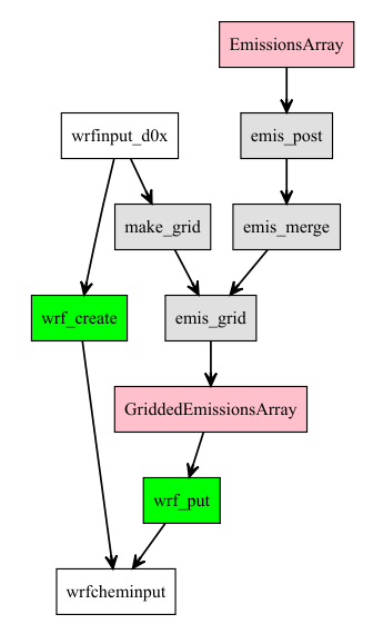
Figure 9.1: Generation of wrfchem inputs using GriddedEmissionsArray

Example

9.1.1 Creating a WRF-Chem input file

The emission file is generated with traffic simulation from the Traffic Engineering Company (CET) for 2012, which consists in traffic flow for morning rush hour of Light-Duty Vehicles (LDV). The emission factors are the data fe2015 and the wrfinput comes from the eixport package. Let’s go:

9.1.1.1 0) Network

The object net has a class SpatialLinesDataFrame; we transform it into a sf object. The length of the road is the field ‘lkm’ in the object net, which is in km but has no units. We must add the right units to use vein

require(vein)
require(sf)
require(units)
net <- readRDS("figuras/net.rds")
class(net)
net <- sf::st_as_sf(net)
net[1, ]
net$lkm <- units::set_units(st_length(net), km)

9.1.1.2 1) Vehicular composition

In this case, the vehicular composition consists in only to vehicles, Passenger Cars using Gasoline with 25% of Ethanol and Light Trucks consuming Diesel with 5% od biodiesel. Also, the emission factors cover \(CO\). The temporal distribution will cover only one hour.

PC_E25 <- age_ldv(net$ldv)

9.1.1.3 2) Emission factors

The emission factors used comes from CETESB (2015), which are constant by the age of use. In practice, this data.frame is like an Excel spreadsheet. Then, the constructor function EmissionFactorsList convert our numeric vector, which is the column of our data.frame, into the required type of object of the emis function. Parenthesis was added to print the objects in one line.

data(fe2015)
a <- fe2015[fe2015$Pollutant == "CO", "PC_G"]
(EF_CO_PC_E25 <- EmissionFactorsList(a))

9.1.1.4 3) Estimation of emissions

The estimation of emissions is in the following code chunk in a simplified way, where they are aggregated.

data(profiles)
emi <- emis(veh = PC_E25, lkm = net$lkm, ef = EF_CO_PC_E25,
             profile = profiles$PC_JUNE_2012)

9.1.1.5 4) Post-estimations

The resulting emissions array emi is now processed with emis_post.

co_street <- emis_post(arra = emi, by = "streets_wide",
                       net = net)

9.1.1.5.1 4a WRFChem input file with `eixport`

Now it is time to generate the emissions grid. To create a wrfchem input file, we need a wrfinput file. In this case, the wrfinput covers a broader area of the emissions, located in São Paulo, Brazil. The wrfinput file is available from the R package eixport.

wrf <- paste(system.file("extdata", package = "eixport"),
             "/wrfinput_d02", sep="")
g  <- make_grid(wrf)

## path to wrfinput

## using grid info from: /home/sergio/R/x86_64-pc-linux-gnu-library/3.5/eixport/extdata/wrfinput_d02 
## Number of lat points 51
## Number of lon points 63

plot(st_geometry(g), axes = TRUE)
plot(st_geometry(co_street), add = TRUE, lwd = 0.1)

Notice that we create a grid from the path to wrfinput, there is a message with Number of lat points 51 and Number of long points 63. This information is critical for later conversions. Now that we have the street emissions and the grid, we can obtain our gridded emissions:

gCO <- emis_grid(spobj = co_street, g = g)

## Sum of street emissions 1845699895.43
## Sum of gridded emissions 1845699895.43

# names(gCO)
# gCO$geometry

This function requires the package lwgeom when the data is in latitude and longitude degrees. There are some messages about the total emissions of street and grid. This was made in order to ensure that emis_grid is conservative. The resulting object gCO is an sf object of POLYGON. In order to plot the emissions, i selected the emissions above 1, because it is easier to see the plot. If we plot the gridded emissions, we will see:

gCO$V9 <- gCO$V9*(12 + 16)^-1
plot(gCO[gCO$V9 >1, "V9"], axes = TRUE,  nbreaks = 50,
     pal = cptcity::cpt(colorRampPalette = T),
     main = "Emissions of CO at 08:00 (mol/h)", lwd = 0.2)

Figure 9.2: Gridded emissions (mol/h)

The emissions are mostly distributed into main roads, as expected. The next step is to create the GriddedEmissionsArray that will be inputted into the eixport functions. The GriddedEmissionsArray is a constructor function that reads class, SpatialPolygonDataFrame, sf of POLYGONs, a data.frame or a matrix to create an Array of the gridded emissions. The dimensions are lat, long, mass and time. Therefore, it is important to know the number of lat and long points!

gCOA <- GriddedEmissionsArray(x = gCO, cols = 63,
                              rows = 51, times = 168)

## This GriddedEmissionsArray has:
##  51 lat points
##  63 lon points
##  168 hours

plot(gCOA, col = cptcity::cpt())

Figure 9.3: GriddedEmissionsArray (mol/h)

The image is similar to the plot of the gridded emissions, which means that it is correct. Now we can input our newly created object gCOA into the wrfchem input file, but first, we need to create it. This is done using the eixport functions. We first load the library eixport. Then load the data emis_opt which has the emissions options for WRFchem. In this case, we are creating a wrfchem input file with 40 pollutants, with 0.

library(eixport)
data(emis_opt)
emis_opt[["ecb05_opt1"]]
wrf_create(wrfinput_dir = system.file("extdata", 
                                      package = "eixport"),
           wrfchemi_dir = tempdir(),
           frames_per_auxinput5 = 168,
           domains = 2,
           variaveis = emis_opt[["ecb05_opt1"]],
           verbose = F)

The wrfchemi input file was created on a temporary directory with the function tempdir. Now we can input our GriddedEmissionsArray into our new wrfchem input file.

f <- list.files(path = tempdir(), full.names = T, 
                pattern = "wrfchemi_d02")
f
wrf_put(file = f, name = "E_CO", POL = gCOA)

Then, we check our resulting NetCDF file plotting the emissions we just put.

wrf_plot(f, "E_CO")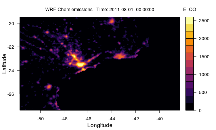

Figure 9.4: Wrfchem input file (NetCDF) (mol/h)

9.1.1.5.2 4b WRFChem input file with `emis_wrf`

emis_wrf creates a data.frame with columns lat, long, id, pollutants, local time and GMT. This dataframe has the proper format to be used with WRF assimilation system: “assimilation System 4 WRF (AS4WRF, Vara-Vela (2013))

args(emis_wrf)

## function (sdf, nr = 1, dmyhm, tz, crs = 4326, islist, utc) 
## NULL

where:

sdf: Gridded emissions, which can be a SpatialPolygonsDataFrame, or a list of SpatialPolygonsDataFrame, or an sf object of “POLYGON”. The user must enter a list with 36 SpatialPolygonsDataFrame with emissions for the mechanism CBM-Z.
nr: Number of repetitions of the emissions period
dmyhm: String indicating Day Month Year Hour and Minute in the format “d-m-Y H:M” e.g., “01-05-2014 00:00” It represents the time of the first hour of emissions in Local Time
tz: Time zone as required in for function as.POSIXct
crs: Coordinate reference system, e.g: “+init=epsg:4326”. Used to transform the coordinates of the output
islist: logical value to indicate if sdf is a list or not
utc: ignored.

In this case, we can use our gridded emissions directly here:

gCO$id <- NULL
df <- emis_wrf(sdf = gCO, dmyhm = "06-10-2014 00:00",
               tz = "America/Sao_Paulo", islist = FALSE)
df[1, ]

##  id   long      lat   pol  time_lt      
##  1  -47.418  -24.350  CO  2014-10-06

Then you must export this data.frame into a .txt file. You must include the number of columns to match your lumped species and also take out the columns time_lt, time_utc and dutch. These three columns are just informative.

df <- df[,1:4]
write.table(x = df, file = tempfile(), sep = "\t",
            col.names = TRUE, row.names = FALSE)

To generate the wrfchem input file, you must have the resulting .txt file, a wrfinput file with the same grid spacing, the NCL script AS4WRF and a namelist. AS4WRF and the namelist can be obtained contacting angel.vela@iag.usp.br.

There is also a new approach with the model EmissV (Schuch et al. 2018), which estimates vehicular emissions and generates inputs for air quality models. EmissV (Schuch, Ibarra-Espinosa, and Dias de Freitas 2018) is an R package designed to work gridded data, which can also process emissions global dataset EDGAR (EJ-JRC/PBL 2016). the emissions.

References

Grell, Georg A, Steven E Peckham, Rainer Schmitz, Stuart A McKeen, Gregory Frost, William C Skamarock, and Brian Eder. 2005. “Fully Coupled ‘Online’ Chemistry Within the Wrf Model.” Atmospheric Environment 39 (37). Elsevier: 6957–75.

Vara-Vela, A., M. F. Andrade, P. Kumar, R. Y. Ynoue, and A. G. Muñoz. 2016. “Impact of Vehicular Emissions on the Formation of Fine Particles in the São Paulo Metropolitan Area: A Numerical Study with the Wrf-Chem Model.” Atmos. Chem. and Phys. 16: 777–97. doi:10.5194/acp-16-777-2016.

Boulder, Colorado: UCAR/NCAR/CISL/TDD. 2017. “The Ncar Command Language (Ncl)(version 6.4. 0).” http://dx.doi.org/10.5065/D6WD3XH5.

Ibarra, Sergio, Amanda Rehein, Angel Vara-Vela, and Rita Ynoue. 2015. Simulation for the Metropolitan Region of Porto Alegre. Edited by Sergio Ibarra, Amanda Rehein, Angel Vara-Vela, and Rita Ynoue.

Ibarra, Sergio, Rita Ynoue, and Angel Vara-Vela. 2015. Emissions Inventory and Atmospheric Simulation of 58 Urban Centers of South America. Edited by Sergio Ibarra, Rita Ynoue, and Angel Vara-Vela.

Ibarra-Espinosa, Sergio, Daniel Schuch, and Edmilson Dias de Freitas. 2018. “Eixport: An R Package to Export Emissions to Atmospheric Models.” The Journal of Open Source Software. doi:10.21105/joss.00607.

Ibarra-Espinosa, Sergio, Daniel Schuch, and Edmilson Dias de Freitas. 2017. Eixport: An R Package to Export Emissions to Atmospheric Models. https://CRAN.R-project.org/package=eixport.

Freitas, Edmilson, Leila Martins, Pedro Silva Dias, and María de Fátima Andrade. 2005. “A Simple Photochemical Module Implemented in Rams for Tropospheric Ozone Concentration Forecast in the Metropolitan Area of São Paulo, Brazil: Coupling and Validation.” Atmospheric Environment 1 (39). Elsevier: 6352–61.

Snyder, Michelle G., Akula Venkatram, David K. Heist, Steven G. Perry, William B. Petersen, and Vlad Isakov. 2013. “RLINE: A Line Source Dispersion Model for Near-Surface Releases.” Atmospheric Environment 77: 748–56. doi:https://doi.org/10.1016/j.atmosenv.2013.05.074.

CETESB. 2015. “Emissões Veiculares No Estado de São Paulo 2014.”

Vara-Vela, A. 2013. “Avaliação Do Impacto Da Mudança Dos Fatores de Emissão Veicular Na Formação de Ozônio Troposférico Na Região Metropolitana de São Paulo(RMSP).” PhD thesis, São Paulo, Brazil: Instituto de Astronomia, Geofísica e Ciências Atmosféricas, Universidade de São Paulo.

Schuch, Daniel, Sergio Ibarra-Espinosa, Edmilson Drias de Freitas, and Maria de Fatima Andrade. 2018. “EmissV: A Preprocessor for Wrf-Chem Model.” Journal of Atmospheric Science Research 1 (2): 35–45. http://ojs.bilpublishing.com/index.php/jasr.

Schuch, Daniel, Sergio Ibarra-Espinosa, and Edmilson Dias de Freitas. 2018. “EmissV: An R Package to Create Vehicular and Other Emissions by Top-down Methods to Air Quality Models.” The Journal of Open Source Software. http://joss.theoj.org/papers/10.21105/joss.00662.

EJ-JRC/PBL. 2016. “Emission Database for Global Atmospheric Research (Edgar), Release Edgar V4.3.1_v2 (1970 - 2010).” http://edgar.jrc.ec.europa.eu.