Chapter 8 Speciation
The speciation for emissions is a very important part that deserves a only chapter on this book. VEIN initially covered speed functions emission factors of CO, HC, NOx, PM and Fuel Consumption (FC). But currently, the the pollutants covered are:
- Criteria: “CO”, “NOx”, “HC”, “PM”, “CH4”, “NMHC”, “CO2”, “SO2”, “Pb”, “FC” (Fuel Consumption).
- Polycyclic Aromatic Hydrocarbons (PAH) and Persisten Organic Pollutants (POP): “indeno(1,2,3-cd)pyrene”, “benzo(k)fluoranthene”, “benzo(b)fluoranthene”, “benzo(ghi)perylene”, “fluoranthene”, “benzo(a)pyrene”, “pyrene”, “perylene”, “anthanthrene”, “benzo(b)fluorene”, “benzo(e)pyrene”, “triphenylene”, “benzo(j)fluoranthene”, “dibenzo(a,j)anthacene”, “dibenzo(a,l)pyrene”, “3,6-dimethyl-phenanthrene”, “benzo(a)anthracene”, “acenaphthylene”, “acenapthene”, “fluorene”, “chrysene”, “phenanthrene”, “napthalene”, “anthracene”, “coronene”, “dibenzo(ah)anthracene”
- Dioxins and Furans: “PCDD”, “PCDF”, “PCB”.
- Metals: “As”, “Cd”, “Cr”, “Cu”, “Hg”, “Ni”, “Pb”, “Se”, “Zn”.
- NMHC:
- ALKANES: “ethane”, “propane”, “butane”, “isobutane”, “pentane”, “isopentane”, “hexane”, “heptane”, “octane”, “TWO_methylhexane”, “nonane”, “TWO_methylheptane”, “THREE_methylhexane”, “decane”, “THREE_methylheptane”, “alcanes_C10_C12”, “alkanes_C13”.
- CYCLOALKANES: “cycloalcanes”.
- ALKENES: “ethylene”, “propylene”, “propadiene”, “ONE_butene”, “isobutene”, “TWO_butene”, “ONE_3_butadiene”, “ONE_pentene”, “TWO_pentene”, “ONE_hexene”, “dimethylhexene”.
- ALKYNES:“ONE_butine”, “propine”, “acetylene”.
- ALDEHYDES: “formaldehyde”, “acetaldehyde”, “acrolein”, “benzaldehyde”, “crotonaldehyde”, “methacrolein”, “butyraldehyde”, “isobutanaldehyde”, “propionaldehyde”, “hexanal”, “i_valeraldehyde”, “valeraldehyde”, “o_tolualdehyde”, “m_tolualdehyde”, “p_tolualdehyde”.
- KETONES: “acetone”, “methylethlketone”.
- AROMATICS: “toluene”, “ethylbenzene”, “m_p_xylene”, “o_xylene”, “ONE_2_3_trimethylbenzene”, “ONE_2_4_trimethylbenzene”, “ONE_3_5_trimethylbenzene”, “styrene”, “benzene”, “C9”, “C10”, “C13”.
Also, some Brazilian emission factors and speciations for WRF-Chem, mechanisms: “e_eth”, “e_hc3”, “e_hc5”, “e_hc8”, “e_ol2”, “e_olt”, “e_oli”, “e_iso”, “e_tol”, “e_xyl”, “e_c2h5oh”, “e_ald”, “e_hcho”, “e_ch3oh”, “e_ket”, “E_SO4i”, “E_SO4j”, “E_NO3i”, “E_NO3j”, “E_MP2.5i”, “E_MP2.5j”, “E_ORGi”, “E_ORGj”, “E_ECi”, “E_ECj”, “H2O”.
The speciation of emissions in VEIN can be done with three ways, by selecting the pollutants in ef_speed* functions, another way explicit and the other implicit. The explicit way is by using the function speciate for the specifically available speciation. The implicit way is by adding a percentage value in the argument k in any of the functions of emission factors. The implicit way requires that the user must know the percentage of the species of pollutant.
8.1 Speed functions of VOC species
As mentioned before, the speed function emission factors, currently cover several pollutants. We firstly focus on some PAH and POP.
library(vein)
pol <- c("indeno(1,2,3-cd)pyrene", "benzo(k)fluoranthene",
         "benzo(b)fluoranthene", "benzo(ghi)perylene",
         "fluoranthene", "benzo(a)pyrene")
df <- lapply(1:length(pol), function(i){
  EmissionFactors(ef_ldv_speed("PC", "4S", "<=1400", "G",
                  "PRE", pol[i], x = 10)(10))
})
names(df) <- pol
df
## $`indeno(1,2,3-cd)pyrene`
## 1.03e-06 [g/km]
##
## $`benzo(k)fluoranthene`
## 3e-07 [g/km]
##
## $`benzo(b)fluoranthene`
## 8.8e-07 [g/km]
##
## $`benzo(ghi)perylene`
## 2.9e-06 [g/km]
##
## $fluoranthene
## 1.822e-05 [g/km]
##
## $`benzo(a)pyrene`
## 4.8e-07 [g/km]These pollutants come from Ntziachristos and Samaras (2016) and in this case, are not dependent on speed. I used lapply to iterate in each pollutant at 10 km/h. Now I will show the same example for dioxins and furans.
library(vein)
pol <- c("PCDD", "PCDF", "PCB")
df <- lapply(1:length(pol), function(i){
  EmissionFactors(ef_ldv_speed("PC", "4S", "<=1400", "G",
                   "PRE", pol[i], x = 10)(10))
})
names(df) <- pol
df
## $PCDD
## 1.03e-11 [g/km]
##
## $PCDF
## 2.12e-11 [g/km]
##
## $PCB
## 6.4e-12 [g/km]In the case of nmhc, the estimation is:
library(vein)
pol <- c("ethane", "propane", "butane", "isobutane", "pentane")
df <- lapply(1:length(pol), function(i){
  EmissionFactors(ef_ldv_speed("PC", "4S", "<=1400", "G",
                  "PRE", pol[i], x = 10)(c(10,20,30)))
})
names(df) <- pol
df
## $ethane
## Units: [g/km]
## [1] 0.09934632 0.06062781 0.04524681
##
## $propane
## Units: [g/km]
## [1] 0.02829865 0.01726974 0.01288849
##
## $butane
## Units: [g/km]
## [1] 0.1746087 0.1065580 0.0795247
##
## $isobutane
## Units: [g/km]
## [1] 0.07767076 0.04739993 0.03537478
##
## $pentane
## Units: [g/km]
## [1] 0.10717361 0.06540455 0.04881171Now the same example for one pollutant and several euro standards.
library(vein)
euro <- c("V", "IV", "III", "II","I", "PRE")
df <- lapply(1:length(euro), function(i){
  EmissionFactors(ef_ldv_speed("PC", "4S", "<=1400", "G",
                  euro[i], "benzene")(c(10, 30, 50)))
})
names(df) <- euro
df
## $V
## Units: [g/km]
## [1] 0.0003928819 0.0002194495 0.0001597751
##
## $IV
## Units: [g/km]
## [1] 0.0004864655 0.0004872061 0.0005276205
##
## $III
## Units: [g/km]
## [1] 0.0017465678 0.0008206890 0.0005928019
##
## $II
## Units: [g/km]
## [1] 0.013332523 0.004133087 0.002363304
##
## $I
## Units: [g/km]
## [1] 0.025656752 0.010921829 0.006979341
##
## $PRE
## Units: [g/km]
## [1] 0.4112336 0.1872944 0.12878958.2 Speciate function
The arguments of the function speciate are:
args(vein::speciate)## function (x, spec = "bcom", veh, fuel, eu, show = FALSE,
## list = FALSE, dx) Where,
x: Emissions estimationspec: speciation: The speciations are: “bcom”, tyre“,”break“,”road“,”iag“,”nox" and “nmhc”. ‘iag’ now includes speciation for the use of industrial and building paintings. “bcom” stands for black carbon and organic matter.veh: Type of vehicle: When the spec is “bcom” or “nox” veh can be “PC”, “LCV”, HDV" or “Motorcycle”. When spec is “iag” veh can take two values depending: when the speciation is for vehicles veh accepts “veh”, eu “Evaporative”, “Liquid” or “Exhaust” and fuel “G”, “E” or “D”, when the speciation is for painting, veh is “paint” fuel or eu can be “industrial” or “building” when spec is “nmhc”, veh can be “LDV” with fuel “G” or “D” and eu “PRE”, “I”, “II”, “III”, “IV”, “V”, or “VI”. when spec is “nmhc”, veh can be “HDV” with fuel “D” and eu “PRE”, “I”, “II”, “III”, “IV”, “V”, or “VI”. when spec is “nmhc” and fuel is “LPG”, veh and eu must be “ALL”fuel: Fuel. When the spec is “bcom” fuel can be “G” or “D”. When the spec is “iag” fuel can be “G”, “E” or “D”. When spec is “nox” fuel can be “G”, “D”, “LPG”, “E85” or “CNG”. Not required for “tyre”, “break” or “road”. When the spec is “nmhc” fuel can be G, D or LPG.eu: Euro emission standard: “PRE”, “ECE_1501”, “ECE_1502”, “ECE_1503”, “I”, “II”, “III”, “IV”, “V”, “III-CDFP”,“IV-CDFP”,“V-CDFP”, “III-ADFP”, “IV-ADFP”,“V-ADFP” and “OPEN_LOOP”. When the spec is “iag” accept the values “Exhaust” “Evaporative” and “Liquid”. When the spec is “nox” eu can be “PRE”, “I”, “II”, “III”, “IV”, “V”, “VI”, “VIc”, “III-DPF” or “III+CRT”. Not required for “tyre”, “break” or “road”show: when TRUE shows the row of the table with respective speciationlist: when TRUE returns a list with some elements of the list as the number species of pollutants
As shown before, there is currently 8 type of speciations.
8.3 Black carbon and organic matter
Let’s use the data inside the vein and estimate emissions. The vehicles considered are Light Trucks, assuming all HGV. We are using the 4 stage estimation with the first part arranging traffic data
library(vein)
# 1 Traffic data
data(net)
data(profiles)
data(fe2015)
lt <- age_hdv(net$ldv)
## Average age of age is 17.12## Number of age is 1946.95 * 10^3 vehvw <- temp_fact(net$ldv, profiles$PC_JUNE_2014) +
temp_fact(net$hdv, profiles$HGV_JUNE_2014)
speed <- netspeed(vw, net$ps, net$ffs, net$capacity,
net$lkm, alpha = 1)
# 2 Emission factors
euro <- c("V", rep("IV", 3),
rep("III", 7), rep("II", 7),
rep("I", 5), rep("PRE", 27))
lefd <- lapply(1:50, function(i) {
ef_hdv_speed(v = "Trucks", t = "RT", g = ">32", gr = 0,
eu = euro[i], l = 0.5, p = "PM",
show.equation = FALSE) })
# 3 Estimate emissions
pmd <- emis(veh = lt, lkm = net$lkm, ef = lefd, speed = speed,
profile = profiles$HGV_JUNE_2014)## 32714.53 kg emissions in 24 hours and 7 days# 4 process emissions
# Agreggating emissions by age of use
df <- apply(X = pmd, MARGIN = c(1,2), FUN = sum, na.rm = TRUE)
# euro
dfbcom <- rbind(speciate(df[, 1],
"bcom", "PC", "D", "V"),
speciate(rowSums(df[, 2:4]),
"bcom", "PC", "D", "IV"),
speciate(rowSums(df[, 5:11]),
"bcom", "PC", "D", "III"),
speciate(rowSums(df[, 12:18]),
"bcom", "PC", "D", "II"),
speciate(rowSums(df[, 19:23]),
"bcom", "PC", "D", "I"),
speciate(rowSums(df[, 24:50]),
"bcom", "PC", "D", "PRE"))
dfbcom$id <- 1:1505
bc <- aggregate(dfbcom$BC, by = list(dfbcom$id), sum)
om <- aggregate(dfbcom$OM, by = list(dfbcom$id), sum)
net$BC <- bc[, 2]
net$OM <- om[, 2]Now we have spatial objects of Back Carbon
sp::spplot(net, "BC", scales = list(draw = T),
           main = "Black Carbon [g/168h]",
col.regions = rev(cptcity::cpt()))![Black Carbon [g/168h]](veinbook_files/figure-html/spplotbm-1.svg)
Figure 8.1: Black Carbon [g/168h]
moreover, Organic Matter
sp::spplot(net, "OM", scales = list(draw = T),
           main = "Organic Matter [g/168h]",
col.regions = rev(cptcity::cpt()))![Organic Matter [g/168h]](veinbook_files/figure-html/spplotom-1.svg)
Figure 8.2: Organic Matter [g/168h]
If you are interested in speciate total emissions by age of use not spatial emissions, you could use emis_post with by = "veh" and then aggregate the emissions by standard. Then speciate PM by standard:
dfpm <- emis_post(arra = pmd,  veh = "LT",
                  size = "small", fuel = "D",
                  pollutant = "PM", by = "veh")
dfpm$euro <- euro
dfpmeuro <- aggregate(dfpm$g, by = list(dfpm$euro), sum)
names(dfpmeuro) <- c("euro", "g")
bcom <- as.data.frame(sapply(1:6, function(i){
  speciate(dfpmeuro$g[i], "bcom", "PC", "D", dfpmeuro$euro[i])
}))
names(bcom) <- dfpmeuro$euro
And the resulting speciation is:
| BC | OM | |
|---|---|---|
| I | 6826527.4 [g/h] | 2730611.0 [g/h] |
| II | 5313757.9 [g/h] | 1222164.3 [g/h] |
| III | 3321183.0 [g/h] | 498177.5 [g/h] |
| IV | 155078.7 [g/h] | 20160.2 [g/h] |
| PRE | 6700527.8 [g/h] | 4690369.5 [g/h] |
| V | 10369.3 [g/h] | 20738.5 [g/h] |
8.4 Tyre wear, breaks wear and road abrasion
Tire, break and road abrasions come from Ntziachristos and Boulter (2009). Tires consist of a complex mixture of rubber, which after the user starts to degrade. Indeed, when the driving cycle is more aggressive, higher is tire mass emitted from the tire, with tire wear emission factors higher in HDV than LDV. Break wear emits mass and with more aggressive driving, more emissions.
The input are wear emissions in Total Suspended Particles (TSP) ,as explained in section @ref(#ew). The speciation consists in 60% PM10, 42% PM2.5, 6% PM1 and 4.8% PM0.1. Now, a simple example for TP adspeciation:
library(vein)
data(net)
data(profiles)
pro <- profiles$PC_JUNE_2012[, 1] # 24 hours
pc_week <- temp_fact(net$ldv+net$hdv, pro)
df <- netspeed(pc_week, net$ps, net$ffs, net$capacity,
               net$lkm, alpha = 1)
ef <- ef_wear(wear = "tyre", type = "PC", speed = df)
emit <- emis_wear(veh = age_ldv(net$ldv,
                                name = "VEH"), speed = df,
                  lkm = net$lkm, ef = ef, profile =  pro)
## Average age of VEH is 11.17## Number of VEH is 1946.95 * 10^3 vehemib <- emis_wear(what = "break",
veh = age_ldv(net$ldv, name = "VEH"),
lkm = net$lkm, ef = ef,
profile = pro, speed = df)## Average age of VEH is 11.17
## Number of VEH is 1946.95 * 10^3 veh# emit
# emib
emitp <- emis_post(arra = emit, veh = "PC",
size = "ALL", fuel = "G",
pollutant = "TSP", by = "veh")
emibp <- emis_post(arra = emib, veh = "PC",
size = "ALL", fuel = "G",
pollutant = "TSP", by = "veh")The estimation covered 24 hours and for simplicity, we are assuming a year with 365 similar days and dividing by 1 million to have t/y. Hence,the speciation is:
library(ggplot2)
tyrew <- speciate(x =  unclass(emitp$g), spec = "tyre")
breakw <- speciate(x =  unclass(emibp$g), spec = "brake")
df <- data.frame(Emis = c(sapply(tyrew, sum),
                          sapply(breakw, sum))*365/1000000)
df$Pollutant <- factor(x = names(tyrew), levels = names(tyrew))
df$Emissions <- c(rep("Tyre", 4), rep("Brake", 4))
ggplot(df, aes(x = Pollutant, y = Emis, fill = Emissions)) +
  geom_bar(stat = "identity", position = "dodge")+
  labs(x = NULL, y = "[t/y]")
Figure 8.3: Break and Tyre emissions (t/y)
It is interesting to see that break emissions are higher than tire wear emissions, and the smaller the diameter, higher the difference, as shown:
| x | |
|---|---|
| PM10 | 1.6593167 |
| PM2.5 | 0.9433433 |
| PM1 | 1.6931803 |
| PM0.1 | 1.6931803 |
The procedure can be used with emis_post with by = streets_wide to obtain the spatial speciation.
8.5 \(NO\) and \(NO_2\)
The speciation of \(NO_X\) into \(NO\) and \(NO2\) depends on the type of vehicle, fuel, and euro standard. The following example will consist in comparing a Gasoline passenger car and a Diesel truck.
library(vein)
data(net)
data(profiles)
propc <- profiles$PC_JUNE_2012[, 1] # 24 hours
prolt <- profiles$PC_JUNE_2012[, 1] # 24 hours
pweek <- temp_fact(net$ldv+net$hdv, pro)
df <- netspeed(pc_week, net$ps, net$ffs,
               net$capacity, net$lkm, alpha = 1)
euro <- c("V", rep("IV", 3),
          rep("III", 7), rep("II", 7),
          rep("I", 5), rep("PRE", 27))
lefpc <- lapply(1:50, function(i) {
  ef_ldv_speed(v = "PC", t = "4S", cc = "<=1400", f = "G",
               eu = euro[i], p = "NOx",
               show.equation = FALSE) })
leflt <- lapply(1:50, function(i) {
  ef_hdv_speed(v = "Trucks", t = "RT",
               g = ">32", gr = 0,
               eu = euro[i], l = 0.5, p = "NOx",
               show.equation = FALSE)
  })
emipc <- emis(veh = age_ldv(net$ldv),
          lkm = net$lkm, ef = lefpc, speed = df,
          profile = profiles$PC_JUNE_2014[, 1])*365/1000000
## Average age of age is 11.17## Number of age is 1946.95 * 10^3 veh## 4097.62 kg emissions in 24 hours and 1 daysemilt <- emis(veh = age_ldv(net$hdv),lkm = net$lkm,
ef = leflt, speed = df,
profile = profiles$HGV_JUNE_2014[, 1])*365/1000000## Average age of age is 11.17## Number of age is 148.12 * 10^3 veh## 14612.67 kg emissions in 24 hours and 1 daysThen, once the emissions are estimated, we will speciate the emissions by euro standard. The estimation covered 24 hours, and for simplicity, we are assuming a year with 365 similar days and dividing by 1 million to have t/y.
df <- rowSums(apply(X = emipc, MARGIN = c(2,3),
                    FUN = sum, na.rm = TRUE))
dfpc <-   rbind(speciate(df[1], "nox", "PC", "G", "V"),
                speciate(df[2:4], "nox", "PC", "G", "V"),
                speciate(df[5:11], "nox", "PC", "G", "V"),
                speciate(df[12:18], "nox", "PC", "G", "V"),
                speciate(df[19:23], "nox", "PC", "G", "V"),
                speciate(df[24:50], "nox", "PC", "G", "V"))
df <- rowSums(apply(X = emipc, MARGIN = c(2,3),
                    FUN = sum, na.rm = TRUE))
dfhdv <-   rbind(speciate(df[1], "nox", "HDV", "D", "V"),
                 speciate(df[2:4], "nox", "HDV", "D", "V"),
                 speciate(df[5:11], "nox", "HDV", "D", "V"),
                 speciate(df[12:18], "nox", "HDV", "D", "V"),
                 speciate(df[19:23], "nox", "HDV", "D", "V"),
                 speciate(df[24:50], "nox", "HDV", "D", "V"))

df <- data.frame(rbind(sapply(dfpc, sum), sapply(dfhdv, sum)))
row.names(df) <- c("PC", "HGV")
knitr::kable(df, caption = "NO2 and NO speciation (t/y)")| NO2 | NO | |
|---|---|---|
| PC | 44.8689 | 1450.761 |
| HGV | 179.4756 | 1316.154 |
8.6 Volatile organic compounds: nmhc
nmhc was shown earlier in this chapter, but they can also be used to speciate objects, resulting in all species at once. The speciation of NMHC must be applied to NMHC. However, the emission guidelines of Ntziachristos and Samaras (2016) does not show specific emission factor of NMHC and the suggested procedure is subtract the \(CH_4\) from the \(HC\). I included this aspect in VEIN with ef_speed* functions to return NMHC directly.
library(vein)
data(net)
data(profiles)
propc <- profiles$PC_JUNE_2012[, 1] # 24 hours
pweek <- temp_fact(net$ldv+net$hdv, propc)
df <- netspeed(pweek, net$ps, net$ffs, net$capacity,
               net$lkm, alpha = 1)
euro <- c("V", rep("IV", 3),
          rep("III", 7), rep("II", 7),
          rep("I", 5), rep("PRE", 27))
lefpc <- lapply(1:50, function(i) {
  ef_ldv_speed(v = "PC", t = "4S", cc = "<=1400", f = "G",
               eu = euro[i], p = "NMHC",
               show.equation = FALSE)})
euro <- c("V", rep("IV", 3), rep("III", 7),
rep("II", 7), rep("I", 5), rep("PRE", 27))
lefpc <- lapply(1:length(euro), function(i) {
ef_ldv_speed(v = "PC", t = "4S", cc = "<=1400", f = "G",
eu = euro[i], p = "HC",
show.equation = FALSE) })
enmhc <- emis(veh = age_ldv(net$ldv), lkm = net$lkm,
ef = lefpc, speed = df,
profile = profiles$PC_JUNE_2014[, 1])## Average age of age is 11.17## Number of age is 1946.95 * 10^3 veh## 3030.65 kg emissions in 24 hours and 1 daysdf_enmhc <- emis_post(arra = enmhc, veh = "PC",
size = "ALL", fuel = "G",
pollutant = "NMHC", by = "veh")
# assuming all euro I
spec <- speciate(x = as.numeric(df_enmhc$g),
spec = "nmhc", veh = "LDV",
fuel = "G", eu = "I")
names(spec)## [1] "ethane" "propane"
## [3] "butane" "isobutane"
## [5] "pentane" "isopentane"
## [7] "hexane" "heptane"
## [9] "octane" "TWO_methylhexane"
## [11] "nonane" "TWO_methylheptane"
## [13] "THREE_methylhexane" "decane"
## [15] "THREE_methylheptane" "alcanes_C10_C12"
## [17] "alkanes_C13" "cycloalcanes"
## [19] "ethylene" "propylene"
## [21] "propadiene" "ONE_butene"
## [23] "isobutene" "TWO_butene"
## [25] "ONE_3_butadiene" "ONE_pentene"
## [27] "TWO_pentene" "ONE_hexene"
## [29] "dimethylhexene" "ONE_butine"
## [31] "propine" "acetylene"
## [33] "formaldehyde" "acetaldehyde"
## [35] "acrolein" "benzaldehyde"
## [37] "crotonaldehyde" "methacrolein"
## [39] "butyraldehyde" "isobutanaldehyde"
## [41] "propionaldehyde" "hexanal"
## [43] "i_valeraldehyde" "valeraldehyde"
## [45] "o_tolualdehyde" "m_tolualdehyde"
## [47] "p_tolualdehyde" "acetone"
## [49] "methylethlketone" "toluene"
## [51] "ethylbenzene" "m_p_xylene"
## [53] "o_xylene" "ONE_2_3_trimethylbenzene"
## [55] "ONE_2_4_trimethylbenzene" "ONE_3_5_trimethylbenzene"
## [57] "styrene" "benzene"
## [59] "C9" "C10"
## [61] "C13"8.7 The speciation iag
The Carbon Bond Mechanism Z (1999) is a lumped-structure mechanism.
Citing:
**“it is currently unfeasible to treat the organic species individually in a regional or global chemistry model for three primary reasons:**
- (1) limited computational resources, - (2) lack of detailed speciated emissions inventories, and - (3) lack of kinetic and mechanistic information for all the species and their reaction products.
Thus there exists a need for a condensed mechanism that is capable of describing the tropospheric hydrocarbon chemistry with reasonable accuracy, sensitivity, and speed at regional to global scales.
The research in this aspect is intense and out of the scope of this book. However, it is vital that the user who intends to performs an atmospheric simulation to understand this why it is essential to speciate the emissions and what represent each group.
A popular air quality model nowadays is the Weather Research and Forecasting model coupled to Chemistry (WRF-Chem) (Grell et al. 2005) https://ruc.noaa.gov/wrf/wrf-chem/and the Emissions Guide (https://ruc.noaa.gov/wrf/wrf-chem/Emission_guide.pdf).
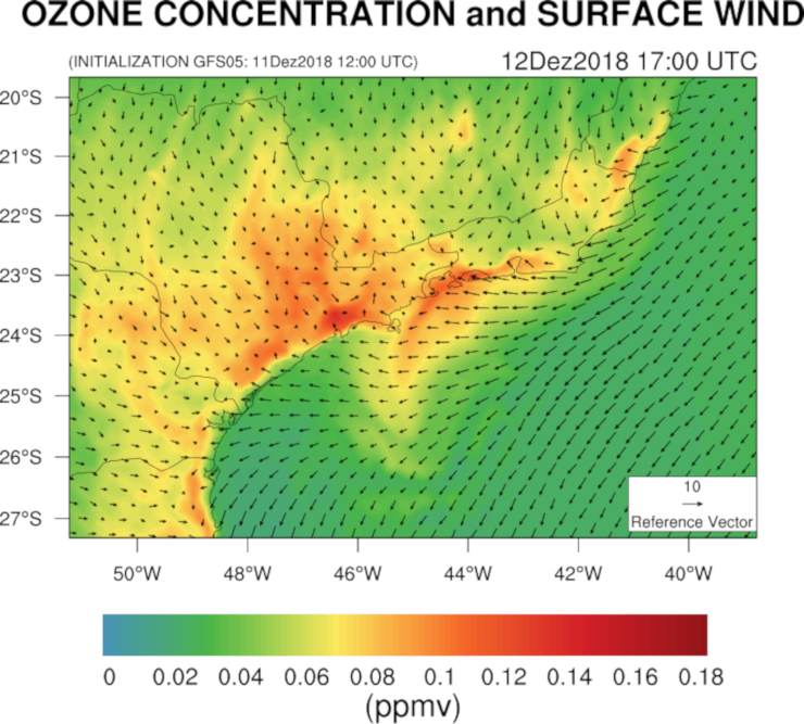
The speciation iag splits the NMHC into the lumped groups for the mechanism CMB-Z. The name iag comes from the Institute of Astronomy, Geophysics and Atmospheric Sciences (IAG, http://www.iag.usp.br/) from the University of São Paulo (USP). The Department of Atmospheric Sciences (DAC) of IAG has measure and model air quality models for several years. There are several scientific productions such as: Nogueira et al. (2015), Hoshyaripour et al. (2016), Andrade et al. (2017), Freitas et al. (2005), Martins et al. (2006), Pérez-Martinez et al. (2014), Ulke and Andrade (2001), Vivanco and Fátima Andrade (2006), Boian and Andrade (2012), Fatima Andrade et al. (2012), Andrade et al. (2015), Vara-Vela et al. (2016), Rafee (2015), Ibarra-Espinosa et al. (2017). The following figure shows an air quality simulation over South East Brazil from DAC/IAG/USP.
Some of these papers show measurements in tunnels and fuel. The speciation iag it is based on these experiments, and the last versions, covers an update during 2015 so that the exhaust emissions speciation is more representative of Brazilian gasoline, which means?
** THE SPECIATION IAG IS BASED ON BRAZILIAN MEASUREMENTS**
Moreover, the user who wants to apply it outside Brazil should be ensured, that the fleet and fuel are compatible. As that will be hard to accomplish, I can say that this speciation is for and to be used in Brazil, even more, in São Paulo.
The currently speciation iag is:
| NMHC | GEX | GEV | GLIQ | EEX | EEV | ELIQ | DEX |
|---|---|---|---|---|---|---|---|
| e_eth | 0.23 | 0.02 | 0.00 | 0.00 | 0.00 | 0.00 | 0.00 |
| e_hc3 | 0.36 | 0.24 | 0.02 | 0.00 | 0.00 | 0.00 | 0.05 |
| e_hc5 | 0.13 | 0.45 | 0.16 | 0.00 | 0.00 | 0.00 | 0.06 |
| e_hc8 | 0.06 | 0.00 | 0.19 | 0.05 | 0.00 | 0.00 | 0.30 |
| e_ol2 | 0.48 | 0.04 | 0.00 | 0.13 | 0.00 | 0.00 | 0.32 |
| e_olt | 0.20 | 0.20 | 0.08 | 0.00 | 0.00 | 0.00 | 0.39 |
| e_oli | 0.13 | 0.46 | 0.18 | 0.00 | 0.00 | 0.00 | 0.00 |
| e_iso | 0.01 | 0.00 | 0.00 | 0.00 | 0.00 | 0.00 | 0.00 |
| e_tol | 0.12 | 0.08 | 0.05 | 0.01 | 0.00 | 0.00 | 0.24 |
| e_xyl | 0.22 | 0.00 | 0.12 | 0.01 | 0.00 | 0.00 | 0.01 |
| e_c2h5oh | 0.31 | 0.35 | 0.61 | 1.52 | 2.17 | 2.17 | 0.00 |
| e_hcho | 0.11 | 0.00 | 0.00 | 0.13 | 0.00 | 0.00 | 0.32 |
Where G is the gasohol, or gasoline blended with 25% of Ethanol, E is 100% ethanol and D is diesel with 5% of biodiesel. EX means exhaust, EV are the evaporative emissions and LIQ the liquid emissions.
The arguments of the function speciate take the following form:
x: Emissions estimation, it is recommended that x are griddded emissions from NMHC.spec:iag. Alternatively, you can put any name of the following: “e_eth”, “e_hc3”, “e_hc5”, “e_hc8”, “e_ol2”, “e_olt”, “e_oli”, “e_iso”, “e_tol”, “e_xyl”, “e_c2h5oh”, “e_hcho”, “e_ch3oh”, “e_ket”veh: When spec is “iag” veh can take two values depending: when the speciation is for vehicles veh accepts “veh”, eu “Evaporative”, “Liquid” or“Exhaust”fuel: “G”, “E” or “D”.eu: “Exhaust” “Evaporative” or “Liquid”.show: Let this FALSE.list: Let this TRUE so that the result is a list, and each element of the list a lumped specie.
Example:
# Do not run
x <- data.frame(x = rnorm(n = 100, mean = 400, sd = 2))
dfa <- speciate(x, spec = "e_eth", veh = "veh",
                fuel = "G", eu = "Exhaust")
head(dfa)
## e_eth
## 1 0.9259756
## 2 0.9259793
## 3 0.9288054
## 4 0.9270968
## 5 0.9202770
## 6 0.9375046df <- speciate(x, spec = "iag", veh = "veh", fuel = "G",
eu = "Exhaust", list = TRUE)
# names(df)
names(df)[1]## [1] "e_eth"df[[1]][1,]## 0.9259756 [mol/h]8.8 The speciation pmiag
The speciation pmiagis also based on IAG studies and applied only for PM2.5 emissions. The speciation splits the PM2.5 in percentages as follow:
| E_SO4i | 0.00770 |
| E_SO4j | 0.06230 |
| E_NO3i | 0.00247 |
| E_NO3j | 0.01053 |
| E_MP2.5i | 0.10000 |
| E_MP2.5j | 0.30000 |
| E_ORGi | 0.03040 |
| E_ORGj | 0.12960 |
| E_ECi | 0.05600 |
| E_ECj | 0.02400 |
When running this speciation, the only two required arguments are x and spec. Also, There is a message that this speciation applies only in gridded emissions, because the unit must be in flux \(g/km^2/h\), and internally are transformed to the required unit $ g/m^2/s$ as:
\[ \frac{g}{(km)^2*h}*\frac{10^6 \mu g}{g}*(\frac{km}{1000m})^2*\frac{h}{3600s}\frac{1}{dx^2}\]
dx is the length of the grid cell. Example:
library(vein)
data(net)
pm <- data.frame(pm = rnorm(n = length(net),
                            mean = 400, sd = 2))
net@data <- pm
g <- make_grid(net, 1/102.47/2) # 500 m
## Number of lon points: 23
## Number of lat points: 19gx <- emis_grid(net, g)## Sum of street emissions 601957.37
## Sum of gridded emissions 601957.37df <- speciate(gx, spec = "pmiag", veh = "veh", fuel = "G",
eu = "Exhaust", list = FALSE, dx = 0.5)## For emissions grid only, emissions must be in g/(Xkm^2)/h## PM.2.5-10 must be calculated as substraction of PM10-PM2.5 to enter this variable into WRFUncomment to see more details.
# names(df)
# head(df)
df[1, 1:6]
## e_so4i e_so4j e_no3i e_no3j e_pm2.5i e_pm2.5j
## 1 0.0014 0.0116 5e-04 0.002 0.0186 0.0559References
Ntziachristos, L, and Z Samaras. 2016. “EMEP/Eea Emission Inventory Guidebook; Road Transport: Passenger Cars, Light Commercial Trucks, Heavy-Duty Vehicles Including Buses and Motorcycles.” European Environment Agency, Copenhagen.
Ntziachristos, L, and P Boulter. 2009. “EMEP/Eea Emission Inventory Guidebook; Road Transport: Automobile Tyre and Break Wear and Road Abrasion.” European Environment Agency, Copenhagen.
Zaveri, Rahul A, and Leonard K Peters. 1999. “A New Lumped Structure Photochemical Mechanism for Large-Scale Applications.” Journal of Geophysical Research: Atmospheres 104 (D23). Wiley Online Library: 30387–30415.
Grell, Georg A, Steven E Peckham, Rainer Schmitz, Stuart A McKeen, Gregory Frost, William C Skamarock, and Brian Eder. 2005. “Fully Coupled ‘Online’ Chemistry Within the Wrf Model.” Atmospheric Environment 39 (37). Elsevier: 6957–75.
Nogueira, Thiago, Kely Ferreira de Souza, Adalgiza Fornaro, Maria de Fatima Andrade, and Lilian Rothschild Franco de Carvalho. 2015. “On-Road Emissions of Carbonyls from Vehicles Powered by Biofuel Blends in Traffic Tunnels in the Metropolitan Area of Sao Paulo, Brazil.” Atmospheric Environment 108. Pergamon: 88–97.
Hoshyaripour, G., G. Brasseur, M.F. Andrade, M. Gavidia-Calderón, I. Bouarar, and R.Y. Ynoue. 2016. “Prediction of Ground-Level Ozone Concentration in São Paulo, Brazil: Deterministic Versus Statistic Models.” Atmospheric Environment 145: 365–75. doi:http://dx.doi.org/10.1016/j.atmosenv.2016.09.061.
Andrade, Maria de Fatima, Prashant Kumar, Edmilson Dias de Freitas, Rita Yuri Ynoue, Jorge Martins, Leila D Martins, Thiago Nogueira, et al. 2017. “Air Quality in the Megacity of São Paulo: Evolution over the Last 30 Years and Future Perspectives.” Atmospheric Environment 159. Elsevier: 66–82. doi:https://doi.org/10.1016/j.atmosenv.2017.03.051.
Freitas, Edmilson, Leila Martins, Pedro Silva Dias, and María de Fátima Andrade. 2005. “A Simple Photochemical Module Implemented in Rams for Tropospheric Ozone Concentration Forecast in the Metropolitan Area of São Paulo, Brazil: Coupling and Validation.” Atmospheric Environment 1 (39). Elsevier: 6352–61.
Martins, Leila D, Maria F Andrade, Edmilson D Freitas, Angelica Pretto, Luciana V Gatti, Édler L Albuquerque, Edson Tomaz, Maria L Guardani, Maria HRB Martins, and Olimpio MA Junior. 2006. “Emission Factors for Gas-Powered Vehicles Traveling Through Road Tunnels in São Paulo, Brazil.” Environ. Sci. Technol. 40 (21). ACS Publications: 6722–9. doi:10.1021/es052441u.
Pérez-Martinez, PJ, RM Miranda, T Nogueira, ML Guardani, A Fornaro, R Ynoue, and MF Andrade. 2014. “Emission Factors of Air Pollutants from Vehicles Measured Inside Road Tunnels in S ao Paulo: Case Study Comparison.” Int. J. Environ. Sci. Te. 11 (8). Springer: 2155–68.
Ulke, Ana G, and M Fátima Andrade. 2001. “Modeling Urban Air Pollution in Sao Paulo, Brazil: Sensitivity of Model Predicted Concentrations to Different Turbulence Parameterizations.” Atmospheric Environment 35 (10). Elsevier: 1747–63.
Vivanco, Marta G, and Maria de Fátima Andrade. 2006. “Validation of the Emission Inventory in the Sao Paulo Metropolitan Area of Brazil, Based on Ambient Concentrations Ratios of Co, Nmog and Nox and on a Photochemical Model.” Atmospheric Environment 40 (7). Elsevier: 1189–98.
Boian, Cláudia, and Maria de Fátima Andrade. 2012. “Characterization of Ozone Transport Among Metropolitan Regions.” Revista Brasileira de Meteorologia 27 (2). SciELO Brasil: 229–42.
Fatima Andrade, Maria de, Regina Maura de Miranda, Adalgiza Fornaro, Americo Kerr, Beatriz Oyama, Paulo Afonso de Andre, and Paulo Saldiva. 2012. “Vehicle Emissions and Pm2. 5 Mass Concentrations in Six Brazilian Cities.” Air Quality, Atmosphere & Health 5 (1). Springer: 79–88.
Andrade, Maria de Fatima, Rita Y Ynoue, Edmilson Dias Freitas, Enzo Todesco, Angel Vara Vela, Sergio Ibarra, Leila Droprinchinski Martins, Jorge Alberto Martins, and Vanessa Silveira Barreto Carvalho. 2015. “Air Quality Forecasting System for Southeastern Brazil.” Frontiers in Environmental Science 3. Frontiers: 1–12. doi:10.3389/fenvs.2015.00009.
Vara-Vela, A., M. F. Andrade, P. Kumar, R. Y. Ynoue, and A. G. Muñoz. 2016. “Impact of Vehicular Emissions on the Formation of Fine Particles in the São Paulo Metropolitan Area: A Numerical Study with the Wrf-Chem Model.” Atmos. Chem. and Phys. 16: 777–97. doi:10.5194/acp-16-777-2016.
Rafee, S. A. A. 2015. “Estudo Numerico Do Impacto Das Emissões Veiculares E Fixas Da Cidade de Manaus Nas Concentrações de Poluentes Atmosféricos Da Região Amazônica.” PhD thesis, Londrina: Universidade Tecnologica Federal do Parana.
Ibarra-Espinosa, S., R. Ynoue, S. O’Sullivan, E. Pebesma, M. D. F. Andrade, and M. Osses. 2017. “VEIN V0.2.2: An R Package for Bottom-up Vehicular Emissions Inventories.” Geoscientific Model Development Discussions 2017: 1–29. doi:10.5194/gmd-2017-193.