Chapter 7 Post estimation with emis_post

Once the emissions are estimated we obtained EmissionsArray objects, which as mentioned before, they are arrays with the dimensions streets x age distribution of vehicles x hours x days.

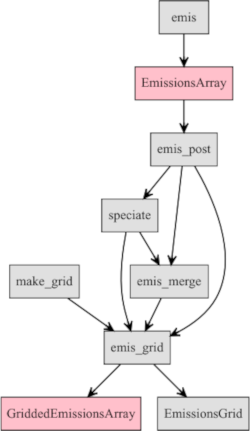
Figure 7.1: Post-emissions

Now the function emis_post reads the EmissionsArray also, convert it to data-frames that are easier to manage.

The arguments of emis_post are:

args(vein::emis_post)

## function (arra, veh, size, fuel, pollutant,
## by = "veh", net) 

Where,

• arra: EmissionsArray obtained with the emis functions. It is an array of emissions 4d: streets x category of vehicles x hours x days or 3d: streets x category of vehicles x hours.
• veh: Character indicating the type of vehicle, for instance: “PC”.
• size: Character indicating the size or weight, for instance: “<1400”, “1400<cc<2000”, “GLP”, “Diesel”.
• fuel: Character indicating fuel, for instance: “Gasoline”, “E_25”, “GLP”, “Diesel”.
• pollutant: Character indicating the pollutant, for instance, “CO”, “NOx”, …
• by: Character indicating the type of output, “veh” for the total vehicular category, “streets_narrow” or “streets_wide”. “streets_wide” or just “streets” returns a dataframe with rows as the number of streets and columns the hours as days*hours considered, e.g., 168 columns as the hours of a whole week and “streets_wide repeats the row number of streets by the hour and day of the week

Let’s create some objects

7.1 Emissions by street

From previous chapters, we worked with Vehicles, EmissionFactors and estimate emissions generating EmissionsArray. Now let’s create an EmissionsArray object.

library(vein)
library(veinreport)

## 
## Attaching package: 'veinreport'

## The following object is masked _by_ '.GlobalEnv':
## 
##     theme_black

library(cptcity)
library(ggplot2)
data(net)
data(profiles)
data(fe2015)
PC_G <- age_ldv(x = net$ldv, name = "PC")

## Average age of PC is 11.17

## Number of PC is 1946.95 * 10^3 veh

# Estimation for 168 hour and local factors
pcw <- temp_fact(net$ldv, profiles$PC_JUNE_2014)
# June is not holliday in southern hemisphere
hdvw <- temp_fact(net$hdv, profiles$HGV_JUNE_2014)
speed <- netspeed(pcw + hdvw, net$ps, net$ffs, 
                  net$capacity, net$lkm, alpha = 1)
a <- fe2015[fe2015$Pollutant=="CO", "PC_G"]
lef <- EmissionFactorsList(a)
E_CO <- emis(veh = PC_G,lkm = net$lkm, ef = lef, 
             speed = speed,
             profile = profiles$PC_JUNE_2014)

## 187546.38 kg emissions in 24 hours and 7 days

Now that we have our EmissionsArray E_CO, we can process it with the function emis_post. The emissions by street are obtained with the argument by = “streets_wide”:

E_CO_STREETS <- emis_post(E_CO, by = "streets_wide")
E_CO_STREETS[1:3, 1:3]

## Result for Emissions 
##                V1             V2              V3
## 1 676.62941 [g/h] 349.0683 [g/h] 206.13032 [g/h]
## 2 259.92480 [g/h] 134.0933 [g/h]  79.18423 [g/h]
## 3  38.10753 [g/h]  19.6594 [g/h]  11.60919 [g/h]

In the version 0.3.17 it was added the capability of returning an spatial object class ‘sf’ with ‘LINESTRING’:

E_CO_STREETS <- emis_post(E_CO, by = "streets_wide", net = net)
class(E_CO_STREETS)

## [1] "sf"         "data.frame"

ggplot(E_CO_STREETS) + geom_sf(aes(colour = as.numeric(V9))) +
  scale_color_gradientn(colours = rev(cpt())) + theme_bw()+
  ggtitle("CO emissions at 08:00 (g/h)")

Figure 7.2: CO emisions of PC (g/h)

Now, if we estimate the NOx emissions of Light Trucks we will a slight different pattern of emissions:

LT <- age_hdv(x = net$hdv, name = "LT")

## Average age of LT is 17.12

## Number of LT is 148.12 * 10^3 veh

efnox <- fe2015[fe2015$Pollutant=="NOx", "LT"]
lef <- EmissionFactorsList(efnox)
E_NOx <- emis(veh = LT, lkm = net$lkm, ef = lef, 
              speed = speed, profile = profiles$PC_JUNE_2014)

## 34029.87 kg emissions in 24 hours and 7 days

E_NOx_STREETS <- emis_post(E_NOx, by = "streets_wide",
                           net = net)
ggplot(E_NOx_STREETS) + geom_sf(aes(colour = as.numeric(V9)))+
  scale_color_gradientn(colours = rev(cpt())) + theme_bw()+
  ggtitle("NOX emissions at 08:00 (g/h)")

Figure 7.3: NOx emisions of LT (g/h)

7.2 Total emissions in data-frames

To obtain the total emissions in data-frame, the same function emis_post is used, but in this case, with the argument by = “veh”. We also need to add arguments of veh for the type of vehicle, size the size or gross weight, fuel and pollutant. The argument net is not required in this case.

E_NOx_DF <- emis_post(arra = E_NOx, veh = "LT",
                      size = "Small", fuel = "B5",
                      by = "veh", pollutant = "NOx")
head(E_NOx_DF, 2)

##     E_NOx              g veh  size fuel pollutant age hour
## 1 E_NOx_1 182.5943 [g/h]  LT Small   B5       NOx   1    1
## 2 E_NOx_2 163.2499 [g/h]  LT Small   B5       NOx   2    1

The resulting object is a data-frame with the name of the input array, and then it has the g/h. Also, the name of the vehicle, the size, fuel, pollutant, age and hour, which is interesting because we can know what the most pollutant vehicle is and at which hour these emissions occurred.

E_NOx_DF[E_NOx_DF$g == max(E_NOx_DF$g), ]

##        E_NOx              g veh  size fuel pollutant age hour
## 517 E_NOx_17 29139.51 [g/h]  LT Small   B5       NOx  17   11

The highest emissions by the hour are of Light Trucks of 17 years of use at hour 11 on local time. However, it is possible to get more interesting insights into the data. The data can be aggregated by age, hour or plot all together as shown in Fig. 7.6. The highest emissions occurred between 17 and 27 years of use. This figure also shows the effect of emissions standards introduced in different years.

df <- aggregate(E_NOx_DF$g, by = list(E_NOx_DF$hour), sum)
plot(df, type = "b", pch = 16, xlab = "hour", ylab = "NOx (g/h)")

Figure 7.4: NOx emissions of LT by hour

library(ggplot2)
library(veinreport) # theme_black
df <- aggregate(E_NOx_DF$g, by = list(E_NOx_DF$age), sum)
names(df) <- c("Age", "g")
ggplot(df, aes(x = Age, y = as.numeric(g),
               fill = as.numeric(g))) +
  geom_bar(stat = "identity") +
  scale_fill_gradientn(colours = cpt()) + theme_black() +
  labs(x = "Age of use", y = "NOx (g/h)")

Figure 7.5: NOx emissions of LT by age

library(ggplot2)
library(veinreport) # theme_black
ggplot(E_NOx_DF, aes(x = age, y = as.numeric(g), fill= hour))+
  geom_bar(stat = "identity") +
  scale_fill_gradientn(colours = cpt()) + theme_black()+
  labs(x = "Age of use", y = "NOx (g/h)")

Figure 7.6: NOx emissions of LT

7.3 Merging emissions

The function inventory was designed to store the emissions of each type of vehicle in each directory. Hence, it was necessary to create a function that reads and merge the emissions that are in each directory, returning a data-frame os a spatial feature data-frame. The function is emis_merge. Fig. 7.1, emis_merge comes after emis_post or speciate. The arguments of emis_merge are:

args(vein::emis_merge)

## function (pol = "CO", what = "STREETS.rds", 
## streets = T, net, path = "emi", crs, 
## under = "after", ignore = FALSE, as_list = FALSE) 

Where,

• pol: Character. Pollutant.
• what: Character. Word to search the emissions names, “STREETS”, “DF” or whatever name. It is important to include the extension .‘rds’
• streets: Logical. If true, emis_merge reads the street emissions created with emis_post by “streets_wide”, returning an object with class ‘sf’. If false, it reads the emissions data-frame and rbind them.
• net: ‘Spatial feature’ or ‘SpatialLinesDataFrame’ with the streets. It is expected that the number of rows is equal to the number of rows of street emissions. If not, the function stops.
• path: Character. A path where emissions are located
• crs: coordinate reference system in numeric format from http://spatialreference.org/ to transform/project spatial data using sf::st_transform

To see how this functions works, let’s run the example in the inventory function. First, let’s create a project, or in other words, a directory named “YourCity”, into the temporary directory. Then run inventory with the default configuration.

name = file.path(tempdir(), "YourCity")
vein::inventory(name = name, show.main = FALSE)

In my case, the files are in directory /tmp/RtmpfPMf7p/YourCity. Now, if you open the file file main.R, you will see:

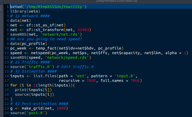
This script starts with setwd function, Then the first section is the network, where the user reads and prepares the traffic information. Then the second section runs a script which runs the age functions for the default vehicular composition of the inventory function. The third section estimates the emissions by running each input.R file inside the directory est The fourth section, creates a grid and run the script post.R is shown below:

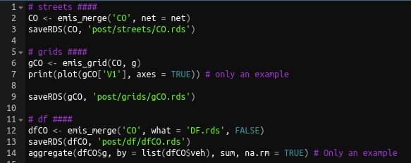
The function emis_merge shown in line 2 is designed to read all the files with names CO and the default argument what is “STREETS.rds”, for instance, PC_GASOLINE_CO_STREETS.rds. Hence, this function reads all the files under that condition. The other argument is streets with default value of TRUE, meaning that the function now knows that the resulting object must be a spatial network, and the net argument is already calling the net object part of the VEIN data, the function merges all the objects summing the emissions of all vehicle street by street. The resulting object is a spatial “LINESTRING” class of sf. This function assumes that emissions files are data.frames and no tests have been made to see if this function would read work sf objects.

On the other hand, the line 12 also runs all the emissions files whose names include the word CO, but also including the words “DF.rds”, which are the files from emis_post with argument by equals to “veh”. In this case, it reads and merges the data-frames and prints the sum emissions by pollutant.

Sourcing the file main.R runs each line of this script, estimating emissions and producing some plots.

source(paste0(name, "/main.R"))

7.4 Creating grids

Once we have processed our emissions array with emis_post and we have spatial emissions, we can then create grids and allocate our emissions into the grids. Let’s check the function make_grid first:

args(vein::make_grid)

## function (spobj, width, height = width, polygon, crs = 4326, 
##     ...) 
## NULL

This function initially used an sp approach. However, now uses an sf approach for creating the grid. The arguments are pretty much the same with the sf::st_make_grid with the exception that is focused in returning polygons with coordinates at centroids of each cell. Therefore, the arguments height and polygon are deprecated. Let’s create a grid for our net.

library(vein)
library(sf)

## Linking to GEOS 3.6.2, GDAL 2.2.3, PROJ 4.9.3

data(net)
net <- st_transform(st_as_sf(net), 31983)
g <- make_grid(spobj = net, width = 500)

## Number of lon points: 23
## Number of lat points: 21

class(g)

## [1] "sf"         "data.frame"

plot(g$geometry, axes = TRUE)
plot(net$geometry, add = TRUE)

Figure 7.7: Grid with spacing of 500 mts

The class of net is SpatialLinesDataFrame, which is converted to sf. Then, as the coordinate reference system of the net is WGS84 with epsg 4326, we are transforming to UTM to create a grid with a grid spacing of 500 m. The class of the grid object, g is “sf data.frame”.

7.5 Gridding bottom-up emissions with emis_grid

The functionemis_grid allocates emissions proportionally to each grid cell. The process is performed by the intersection between geometries and the grid. It means that requires “sr” according to with your location for the projection. It is assumed that spobj is a spatial*DataFrame or an “sf” with the pollutants in data. This function returns an object class “sf”.

Before sf era, i tried to useraster::intersect which imports rgeos and took ages. Then I started to use QGIS Development Team (2017) (https://www.qgis.org), and later the R package Muenchow, Schratz, and Brenning (2018) which takes 10 minutes for allocating emissions of the mega-city of São Paulo and a grid spacing of 1 km. 10 min is not bad. However, when sf appeared and also, included the Spatial Indexes (https://www.r-spatial.org/r/2017/06/22/spatial-index.html), it changed the game. A new era started. It took 5.5 seconds. I could not believe it. However, there also some I could accelerate this process importing some data.table Aggregation functions. Now emis_grid can aggregate large spatial extensions. I haven’t tried yet at continental scale. Let’s see the arguments:

args(vein::emis_grid)

## function (spobj, g, sr, type = "lines") 
## NULL

Where,

• spobj : A spatial dataframe of class “sp” or “sf”. When class is “sp” it is transformed to “sf”.
• g: A grid with class “SpatialPolygonsDataFrame” or “sf”.
• sr: Spatial reference, e.g., 31983. It is required if spobj and g are not projected. Please, see http://spatialreference.org/.
• type: type of geometry: “lines” or “points”.

data(net)
net@data <- data.frame(hdv = net[["hdv"]])
g <- make_grid(spobj = net, width = 1/102.47/2)

## Number of lon points: 23
## Number of lat points: 19

netg <- emis_grid(net, g)

## Sum of street emissions 148118
## Sum of gridded emissions 148118

head(netg)

## Simple feature collection with 6 features and 2 fields
## geometry type:  POLYGON
## dimension:      XY
## bbox:           xmin: -46.8066 ymin: -23.62 xmax: -46.77732 ymax: -23.61512
## epsg (SRID):    4326
## proj4string:    +proj=longlat +datum=WGS84 +no_defs
##   id      hdv                       geometry
## 1  1 201.8275 POLYGON ((-46.8066 -23.62, ...
## 2  2 200.6097 POLYGON ((-46.80172 -23.62,...
## 3  3 205.6319 POLYGON ((-46.79684 -23.62,...
## 4  4 224.1988 POLYGON ((-46.79196 -23.62,...
## 5  5 770.9490 POLYGON ((-46.78708 -23.62,...
## 6  6   0.0000 POLYGON ((-46.7822 -23.62, ...

plot(netg["hdv"], axes = TRUE)

Figure 7.8: Spatial grid of HDV traffic 500 mts

The example in this case, showed the allocation of traffic. The resulting object is a sf with the sum of the attributes inside each grid cell. This means that, when the input are street emissions at different hours, it will return gridded emissions at each hour:

E_NOx_STREETS <- emis_post(E_NOx, by = "streets_wide",
                           net = net)
NOxg <- emis_grid(E_NOx_STREETS, g)

## Sum of street emissions 34029872.64
## Sum of gridded emissions 34029872.64

plot(NOxg["V1"], axes = TRUE)

Figure 7.9: NOx emissions for 00:00 [g/h]

7.6 Gridding top-down emissions with emis_dist

When a top-down approach emissions inventory is made, the spatial distribution of emissions must be made considering some proxy. In the case of vehicular emissions, it can be done with data of Open Street Maps, distributing the emissions into the streets. This can be done with the function with the function emis_dist. In general, this function distributes the emissions into a spatial feature on any type, not only lines.

args(vein::emis_dist)

## function (gy, spobj, pro, osm, verbose = TRUE) 
## NULL

Where,

• gy: Numeric; a unique total (top-down) emissions (grams)
• spobj: A spatial dataframe of class “sp” or “sf”. When class is “sp” it is transformed to “sf”.
• pro: Matrix or data-frame profiles, for instance, pc_profile.
• osm: Numeric; vector of length 5, for instance, c(5, 3, 2, 1, 1). The first element covers ‘motorway’ and ‘motorway_link. The second element covers ’trunk’ and ‘trunk_link’. The third element covers ‘primary’ and ‘primary_link’. The fourth element covers ‘secondary’ and ‘secondary_link’. The fifth element covers ‘tertiary’ and ‘tertiary_link’.
• verbose: Logical; to show more info.

Let’s use the package osmdata (Padgham et al. 2017) to download OpenStreetMap data. The process presented in the following code consists of downloading the OpenStreetMap data delimited by the coordinates og the grid g. Then filter only the lines

library(osmdata)

## Data (c) OpenStreetMap contributors, ODbL 1.0. http://www.openstreetmap.org/copyright

library(sf, quietly = T)
osm <- osmdata_sf(
  add_osm_feature(
    opq(bbox = st_bbox(g)),                             
    key = 'highway'))$osm_lines[, c("highway")]
st <- c("motorway", "motorway_link", "
        trunk", "trunk_link", 
        "primary", "primary_link", 
        "secondary", "secondary_link", 
        "tertiary", "tertiary_link")
osm <- osm[osm$highway %in% st, ]
plot(osm, axes = T,  key.width = lcm(4.5))

Figure 7.10: Open street map lines

The we will distribute the total emissions of E_NOx 3.402987310^{7} into this new lines. There is the argument osm, which gives percentage weights to the type of streets in the following order: “motorway”, “trunk”, “primary”, “secondary” and “tertiary” . For instance osm = 5:1 means 33% of emissions into “motorway” because it is 5 / (1 + 2 + 3 + 4 + 5).

estreet <- emis_dist(gy = sum(E_NOx), spobj = osm, verbose = F)
estreet$emission_osm <- emis_dist(gy = sum(E_NOx), 
                                  spobj = osm, 
                                   osm = 5:1, 
                                  verbose = F)$emission
plot(estreet[c("emission")], 
     main = paste0("Emissions with Default distribution: ",
                   round(sum(estreet$emission)), " [g]"), 
     axes = T,pal = cpt(colorRampPalette = T))

Figure 7.11: Emissions distributed into OSM lines

plot(estreet[c("emission_osm")],
          main = paste0("Emission with OSM distribution: ",
                        round(sum(estreet$emission_osm)),
                        " [g]"), axes = T,
     pal = cpt(colorRampPalette = T))

Figure 7.11: Emissions distributed into OSM lines

7.7 Gridding top-down emissions with grid_emis

Another option to distribute top-down emissions consists in the use of the function grid_emis, which does a similar job than emis_dist but cell by cell. This means that the total emissions are distributed inside each grid cell and not one distribution for the whole domain. This function runs a lapply of emis_dist; hence it takes a little bit more time.

args(vein::grid_emis)

## function (spobj, g, sr, pro, osm, verbose = TRUE) 
## NULL

Where,

• spobj: A spatial dataframe of class “sp” or “sf”. When class is “sp” it is transformed to “sf”.
• g: A grid with class “SpatialPolygonsDataFrame” or “sf”. This grid includes the total emissions with the column “emission”. If the profile is going to be used, the column ‘emission’ must include the sum of the emissions for each profile. For instance, if the profile covers the hourly emissions, the column ‘emission’ bust be the sum of the hourly emissions.
• sr: Spatial reference e.g., 31983. It is required if spobj and g are not projected. Please, see http://spatialreference.org/.
• pro: Numeric, Matrix or data-frame profiles, for instance, pc_profile.
• osm: Numeric; vector of length 5, for instance, c(5, 3, 2, 1, 1). The first element covers ‘motorway’ and ‘motorway_link. The second element covers ’trunk’ and ‘trunk_link’. The third element covers ‘primary’ and ‘primary_link’. The fourth element covers ‘secondary’ and ‘secondary_link’. The fifth element covers ‘tertiary’ and ‘tertiary_link’.
• verbose: Logical; to show more info.

It is required that the grid

NOxg <- NOxg[, "V1"]
names(NOxg)[1] <- "emission"
xnet <- grid_emis(osm, NOxg, verbose = F)
plot(xnet, axes = T,pal = cpt(colorRampPalette = T))

Figure 7.12: Use of grid_emis

References

QGIS Development Team. 2017. QGIS Geographic Information System. Open Source Geospatial Foundation. http://qgis.osgeo.org.

Muenchow, Jannes, Patrick Schratz, and Alexander Brenning. 2018. “RQGIS: Integrating R with Qgis for Statistical Geocomputing.” R Journal. https://rjournal.github.io/archive/2017/RJ-2017-067/RJ-2017-067.pdf.

Padgham, Mark, Bob Rudis, Robin Lovelace, and Maëlle Salmon. 2017. “Osmdata.” The Journal of Open Source Software 2 (14). The Open Journal. doi:10.21105/joss.00305.